9 9 2014 Distribution Overlay Graphs in R for Size Data

DistributionOverlayGraphs.R

Jake H

Tue Sep 09 12:57:14 2014

library(ggplot2)
#ggplot2 makes the distribution curve graphs
library(car)
#not sure what car does but I think it works with lattices
library(splitstackshape)

## Loading required package: data.table

#splitstackshape is an easy package that can help you split columns that have delimiters,
#Original CSV file column labelled "Tray" had entries that needed to be split
picsize5=read.csv('ImageJsize4.csv')
#creates dataframe and reads in the CSV file for sizes
picsize6<-concat.split.multiple(picsize5, "Tray", " ")
#splits the Tray column into Tray_1 with Site Number and Tray_2 with Tray number
foys<-subset(picsize6, Date=="2/26/2014"& Site=="Oyster Bay")
#creates a subset data frame for just the size data from February 26th at Oyster Bay
ggplot(foys, aes(x=Length.mm))+geom_density(aes(group=Tray_1, colour=Tray_1, fill=Tray_1),alpha=0.3)

#creates distribution graph overlays for all populations in Feb at Oyster Bay. Looks cool.
fman<-subset(picsize6, Date=="2/26/2014"& Site=="Manchester")
ggplot(fman, aes(x=Length.mm))+geom_density(aes(group=Tray_1, colour=Tray_1, fill=Tray_1),alpha=0.3)

ffid<-subset(picsize6, Date=="2/28/2014"&Site=="Fidalgo")
ggplot(ffid, aes(x=Length.mm))+geom_density(aes(group=Tray_1, colour=Tray_1, fill=Tray_1),alpha=0.3)

#ffid and fman are just repeating the same subset dataframe command
#and then creating distribution overlay graphs for each site

9 8 2014 Kaplan Meier Survival Graphs

Seattle, WA

Mid 50s to Low 70s Mostly Cloudy

Worked through the examples in Statistical Computing as well as an R instruction video which uses the same sample problem as Statistical Computing as seen below.

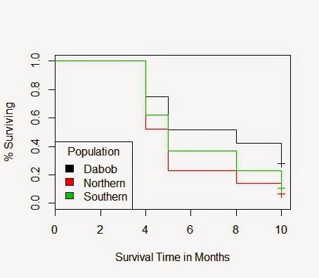
Using my own data from Dabob since the experiment has concluded there, I was able to create a Kaplan Meier graph of survival that compares all three populations at Dabob. This information is censured as there were some animals lost during the experiment. This censorship is marked with a cross at the end as I assumed that when the trays were picked up all animals would be accounted for unless they were definitely missing. The graph is below.

As you can see their seems to be a difference in Survival between the populations. I was not sure if this difference was significant. By modifying the example code from Statistical Computing, I was able to show the mean month of death for each population, the variance for each population, as well as test for significant difference by using survreg. This function helps elucidate any differences between samples that may have extreme variance from one another. In this data set, it showed that there is a significant difference in month of death between all populations. You can see the code for everything and the responses below.

>KMdata3=read.csv("KMdata3.csv")
>attach(KMdata3)
>names(KMdata3)
#[1] "Animal"     "Population" "Death"      "Status"  
>tapply(Death[Status==1],Population[Status==1],mean)
#H        N        S 
#6.034682 5.163311 5.744186 
>tapply(Death[Status==1],Population[Status==1],var)
#H        N        S 
#5.471257 3.280445 4.768906 
>model<-survreg(Surv(Death,Status)~Population,dist="exponential")
> summary(model)
#
#Call:
#  survreg(formula = Surv(Death, Status) ~ Population, dist = "exponential")
#Value Std. Error     z        p
#(Intercept)  2.293     0.0538 42.66 0.00e+00
#PopulationN -0.518     0.0716 -7.24 4.65e-13
#PopulationS -0.361     0.0722 -5.00 5.87e-07
#
#Scale fixed at 1 
#
#Exponential distribution
#Loglik(model)= -3641   Loglik(intercept only)= -3668.9
#Chisq= 55.8 on 2 degrees of freedom, p= 7.6e-13 
#Number of Newton-Raphson Iterations: 3 
#n= 1440 
> plot(fit3, col=c(1:3), xlab="Survival Time in Months", ylab="% Surviving")
> legend("bottomleft", title="Population", c('Dabob','Northern','Southern'), fill=c(1:3))