Primers:
| 1638 | PGE/EP4_FWD | ACAGCGACGGACGATTTTCT | JH | 5/21/2015 | 20 | 55 | O.lurida | Prostaglandin E2 receptor EP4 subtype (PGE receptor EP4 subtype) (PGE2 receptor EP4 subtype) (Prostanoid EP4 receptor) | P32240 | |
| 1637 | PGE/EP4_REV | ATGGCAGACGTTACCCAACA | JH | 5/21/2015 | 20 | 55 | O.lurida | Prostaglandin E2 receptor EP4 subtype (PGE receptor EP4 subtype) (PGE2 receptor EP4 subtype) (Prostanoid EP4 receptor) | P32240 |
Reagent Table:
| Volume | Reactions X116 | |
| Ssofast Evagreen MM | 10 | 1160 |
| FWD Primer | 0.5 | 58 |
| REV Primer | 0.5 | 58 |
| 1:9 cDNA | 9 |
- Added reagents from greatest to least volume
- Vortexed
- Centrifuged briefly
- Pipetted 11 ul Master Mix to each tube
- Pipetted 9 ul of 1:9 cDNA each column using a channel pipetter
- Centrifuged plate at 2000 rpm for 1 minute
- Ran Program Below
Program:
| Step | Temperature | Time |
| Initiation | 95 C | 10 min |
| Elongation | 95 C | 30 sec |
| 60 C | 1 min | |
| Read | ||
| 72 C | 30 sec | |
| Read | ||
| Repeat Elongation 39 times | ||
| Termination | 95 C | 1 min |
| 55 C | 1 sec | |
| Melt Curve Manual ramp 0.2C per sec Read 0.5 C | 55 - 95 C | 30 sec |
| 21 C | 10 min | |
| End |
Plate Layout:
| 1 | 2 | 3 | 4 | 5 | 6 | 7 |
| DNased 42215 HC1 | DNased 42215 NC1 | DNased 42215 SC1 | DNased 42215 HT1 1 | DNased 42215 NT1 1 | DNased 42215 ST1 1 | NTC |
| DNased 42215 HC2 | DNased 42215 NC2 | DNased 42215 SC2 | DNased 42215 HT1 2 | DNased 42215 NT1 2 | DNased 42215 ST1 2 | NTC |
| DNased 42215 HC3 | DNased 42215 NC3 | DNased 42215 SC3 | DNased 42215 HT1 3 | DNased 42215 NT1 3 | DNased 42215 ST1 3 | NTC |
| DNased 42215 HC4 | DNased 42215 NC4 | DNased 42215 SC4 | DNased 42215 HT1 4 | DNased 42215 NT1 4 | DNased 42215 ST1 4 | NTC |
| DNased 42215 HC5 | DNased 42215 NC5 | DNased 42215 SC5 | DNased 42215 HT1 5 | DNased 42215 NT1 5 | DNased 42215 ST1 5 | |
| DNased 42215 HC6 | DNased 42215 NC6 | DNased 42215 SC6 | DNased 42215 HT1 6 | DNased 42215 NT1 6 | DNased 42215 ST1 6 | |
| DNased 42215 HC7 | DNased 42215 NC7 | DNased 42215 SC7 | DNased 42215 HT1 7 | DNased 42215 NT1 7 | DNased 42215 ST1 7 | |
| DNased 42215 HC8 | DNased 42215 NC8 | DNased 42215 SC8 | DNased 42215 HT1 8 | DNased 42215 NT1 8 | DNased 42215 ST1 8 |
Results:
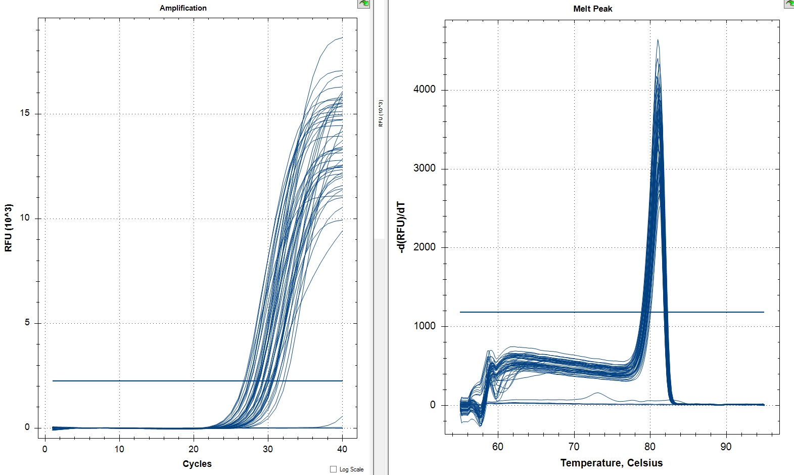
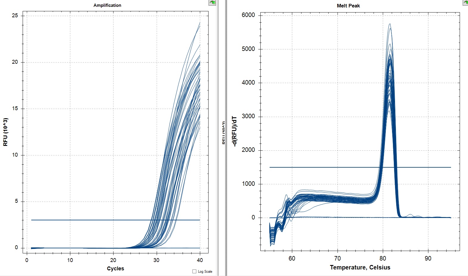
All samples
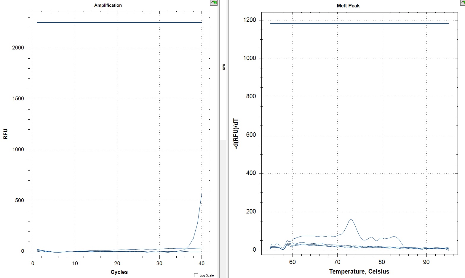
NTCs
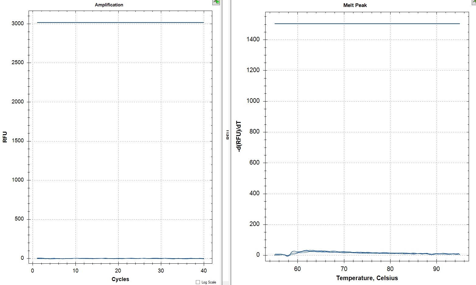
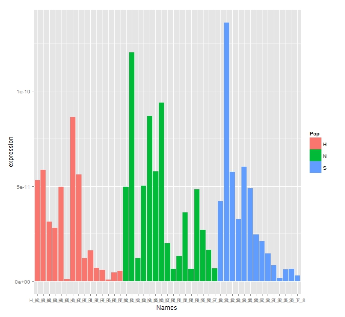
The expression curves look great. There is no amplification in the NTCs which is spectacular. To better understand the data I ran it through my script to generate expression bar graphs, Two Way ANOVA, One Way ANOVA for the populations, and T-Test for the control and treatment in each population.
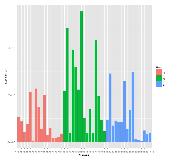
Adjusted Expression Graph
TWO WAY ANOVA and Tukey's TEST
Call:
aov(formula = expression ~ Pop + Treat + Pop:Treat, data = rep2res2)
Terms:
Pop Treat Pop:Treat Residuals
Sum of Squares 1.324664e-21 1.935831e-20 1.181360e-22 2.539439e-20
Deg. of Freedom 2 1 2 39
Residual standard error: 2.551741e-11
Estimated effects may be unbalanced
> TukeyHSD(fit)
Tukey multiple comparisons of means
95% family-wise confidence level
Fit: aov(formula = expression ~ Pop + Treat + Pop:Treat, data = rep2res2)
$Pop
diff lwr upr p adj
N-H 1.298872e-11 -9.354413e-12 3.533185e-11 0.3425329
S-H 5.317103e-12 -1.778535e-11 2.841956e-11 0.8415922
S-N -7.671613e-12 -3.042287e-11 1.507964e-11 0.6920871
$Treat
diff lwr upr p adj
T-C -4.150351e-11 -5.69261e-11 -2.608093e-11 3.1e-06
$`Pop:Treat`
diff lwr upr p adj
N:C-H:C 1.583187e-11 -2.239305e-11 5.405680e-11 0.8140892
S:C-H:C 7.332959e-12 -3.089197e-11 4.555789e-11 0.9921358
H:T-H:C -3.803279e-11 -7.759935e-11 1.533774e-12 0.0656382
N:T-H:C -2.535171e-11 -6.357664e-11 1.287322e-11 0.3678867
S:T-H:C -3.878418e-11 -8.007183e-11 2.503458e-12 0.0762124
S:C-N:C -8.498916e-12 -4.672384e-11 2.972601e-11 0.9846364
H:T-N:C -5.386466e-11 -9.343122e-11 -1.429810e-11 0.0027726
N:T-N:C -4.118358e-11 -7.940851e-11 -2.958655e-12 0.0282920
S:T-N:C -5.461606e-11 -9.590370e-11 -1.332842e-11 0.0038668
H:T-S:C -4.536575e-11 -8.493231e-11 -5.799185e-12 0.0165674
N:T-S:C -3.268467e-11 -7.090960e-11 5.540260e-12 0.1314674
S:T-S:C -4.611714e-11 -8.740479e-11 -4.829501e-12 0.0208893
N:T-H:T 1.268108e-11 -2.688548e-11 5.224764e-11 0.9276071
S:T-H:T -7.513978e-13 -4.328417e-11 4.178138e-11 0.9999999
S:T-N:T -1.343247e-11 -5.472012e-11 2.785517e-11 0.9232037
ONE WAY ANOVA COMPARING POPULATIONS CONTROLS
> fit2<-aov(expression~Pop, data=rep2res2[Treat=="C"])
> fit2
Call:
aov(formula = expression ~ Pop, data = rep2res2[Treat == "C"])
Terms:
Pop Residuals
Sum of Squares 1.004406e-21 2.342257e-20
Deg. of Freedom 2 21
Residual standard error: 3.339701e-11
Estimated effects may be unbalanced
> TukeyHSD(fit2)
Tukey multiple comparisons of means
95% family-wise confidence level
Fit: aov(formula = expression ~ Pop, data = rep2res2[Treat == "C"])
$Pop
diff lwr upr p adj
N-H 1.583187e-11 -2.625788e-11 5.792163e-11 0.6167331
S-H 7.332959e-12 -3.475680e-11 4.942272e-11 0.8996597
S-N -8.498916e-12 -5.058867e-11 3.359084e-11 0.8678189
ONE WAY ANOVA COMPARING POPULATIONS TREATMENT
> fit3<-aov(expression~Pop, data=rep2res2[Treat=="T"])
> fit3
Call:
aov(formula = expression ~ Pop, data = rep2res2[Treat == "T"])
Terms:
Pop Residuals
Sum of Squares 8.423697e-22 1.971827e-21
Deg. of Freedom 2 18
Residual standard error: 1.046642e-11
Estimated effects may be unbalanced
> TukeyHSD(fit3)
Tukey multiple comparisons of means
95% family-wise confidence level
Fit: aov(formula = expression ~ Pop, data = rep2res2[Treat == "T"])
$Pop
diff lwr upr p adj
N-H 1.268108e-11 -1.143704e-12 2.650586e-11 0.0754135
S-H -7.513978e-13 -1.561259e-11 1.410979e-11 0.9908666
S-N -1.343247e-11 -2.785861e-11 9.936614e-13 0.0704802
T-TEST for DABOB
> fit4<-t.test(expression~Treat, data=rep2res2[Pop=="H"])
> fit4
Welch Two Sample t-test
data: expression by Treat
t = 4.1437, df = 7.652, p-value = 0.003565
alternative hypothesis: true difference in means is not equal to 0
95 percent confidence interval:
1.669890e-11 5.936667e-11
sample estimates:
mean in group C mean in group T
4.545505e-11 7.422266e-12
T-TEST for FIDALGO
> fit5<-t.test(expression~Treat, data=rep2res2[Pop=="N"])
> fit5
Welch Two Sample t-test
data: expression by Treat
t = 2.901, df = 9.418, p-value = 0.01678
alternative hypothesis: true difference in means is not equal to 0
95 percent confidence interval:
9.285075e-12 7.308209e-11
sample estimates:
mean in group C mean in group T
6.128693e-11 2.010334e-11
T-TEST for OYSTER BAY
> fit6<-t.test(expression~Treat, data=rep2res2[Pop=="S"])
> fit6
Welch Two Sample t-test
data: expression by Treat
t = 3.5341, df = 7.296, p-value = 0.008921
alternative hypothesis: true difference in means is not equal to 0
95 percent confidence interval:
1.551289e-11 7.672140e-11
sample estimates:
mean in group C mean in group T
5.278801e-11 6.670868e-12
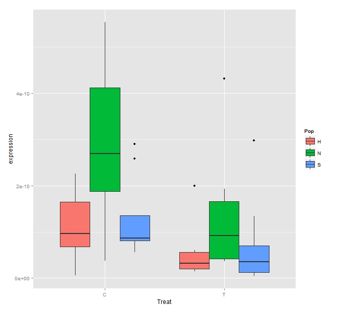
So there isn't a difference between populations but there is a significant difference between treatment and control in all three populations. So PGE/EP4 is suppressed due to heat exposure equally in all populations. This effect can be seen very well in the associated box plot.
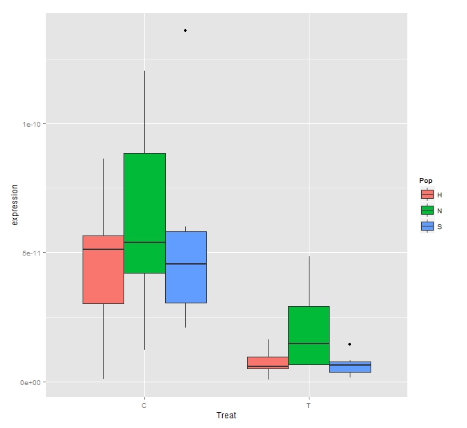
You can see the raw data here.