Resazurin Assays - Selected Juvenile Ruditapes philippinarum Exposed to 40C Acute Heat Stress

INTRO

Steven asked me to perform resazurin assays on “selected” juvenile Ruditapes philippinarum (Manila clam) exposed to 40^oC acute heat stress. The goal of the experiment is to determine if the “selected” clams have higher metabolic activity than control clams when exposed to heat stress.

Data and results are available here:

• https://github.com/RobertsLab/resazurin-assay-development/tree/main/data/clam/20260330-clam-40C-C-vs-S

The section below was knitted from the R Markdown file 00.00-resazurin-20260330-clam-40C-C-vs-S.Rmd (GitHub).

---

1 Background

Control clams (C) compared with selected clams (S) at 40°C using a resazurin metabolic assay. Two plates per family (“blue” and “tweed” shell coloration) were run simultaneously. Clams were placed in 24-well plates submerged in 2.2 mL resazurin working solution (986.66 mL filtered seawater, 2.22 mL resazurin stock, 1.00 mL DMSO, 10.00 mL 100× Penn/Strep & Fungizone). Fluorescence was measured every 30 min on a Synergy HTX (Agilent) plate reader.

See data/clam/20260330-clam-40C-C-vs-S/README.md for full experimental notes.

1.1 Expected inputs

Path	Description
data/clam/20260330-clam-40C-C-vs-S/plate-*-T*.txt	Plate reader fluorescence exports (one file per plate per timepoint)
data/clam/20260330-clam-40C-C-vs-S/layout.csv	Well metadata: plate ID, well ID, blank flag, family/treatment groups, size measurements

1.2 Expected outputs

All outputs are written to output/clam/20260330-clam-40C-C-vs-S/.

File	Description
figures/	All plots generated by this script
auc_all_metrics.csv	Per-individual AUC values for every active measurement metric
auc_summary.csv	Group-level AUC summary statistics (mean, SD, SE, median)
metabolism.csv	Full per-well per-timepoint metabolism data frame
pairwise_stats.csv	Tukey-adjusted pairwise comparisons from AUC linear models

2 Setup

knitr::opts_chunk$set(
  echo = TRUE,         # Display code chunks
  eval = TRUE,        # Evaluate code chunks
  warning = FALSE,     # Hide warnings
  message = FALSE,     # Hide messages
  comment = "",         # Prevents appending '##' to beginning of lines in code output
  results = 'hold'     # Holds output so it's all printed together after code chunk
)

library(tidyverse)
library(pracma)       # trapz()
library(lme4)
library(lmerTest)
library(emmeans)
library(multcompView)
library(cowplot)
library(colorspace)   # qualitative_hcl() for large palettes

3 Helper Functions

normalize_well_id <- function(x) {
  x <- toupper(trimws(x))
  valid <- str_detect(x, "^[A-Z]+[0-9]+$")
  out <- rep(NA_character_, length(x))
  if (!any(valid)) return(out)
  m <- str_match(x[valid], "^([A-Z]+)([0-9]+)$")
  out[valid] <- paste0(m[, 2], as.integer(m[, 3]))
  out
}

parse_time_hr <- function(path) {
  hit <- str_match(basename(path),
                   "(?i)-T([0-9]+(?:\\.[0-9]+)?)\\.txt$")
  as.numeric(hit[, 2])
}

parse_plate_id <- function(path) {
  hit <- str_match(basename(path),
    "(?i)^plate-([A-Za-z0-9-]+)-T[0-9]+(?:\\.[0-9]+)?\\.txt$")
  id <- hit[, 2]
  ifelse(is.na(id), "unknown", id)
}

extract_results_block <- function(lines) {
  results_idx <- which(trimws(lines) == "Results")
  if (length(results_idx) == 0) stop("No Results section found")
  idx <- results_idx[1]
  header_tokens <- str_split(lines[idx + 1], "\\t")[[1]] |> trimws()
  col_ids <- header_tokens[
    header_tokens != "" & str_detect(header_tokens, "^[0-9]+$")]
  j <- idx + 2
  data_lines <- character()
  while (j <= length(lines)) {
    line <- lines[j]
    if (trimws(line) == "") break
    if (!str_detect(line, "^[A-Za-z]\\t")) break
    data_lines <- c(data_lines, line)
    j <- j + 1
  }
  list(col_ids = col_ids, data_lines = data_lines)
}

parse_plate_export <- function(path) {
  lines <- readLines(path, warn = FALSE)
  res <- extract_results_block(lines)

  map_dfr(res$data_lines, function(line) {
    tokens <- str_split(line, "\\t")[[1]] |> trimws()
    tokens <- tokens[tokens != ""]
    row_letter <- tokens[1]
    nums <- suppressWarnings(as.numeric(tokens[-1]))
    valid_idx <- which(!is.na(nums))
    if (length(valid_idx) == 0) return(tibble())
    vals <- nums[valid_idx]
    n <- min(length(vals), length(res$col_ids))
    tibble(
      row_id  = toupper(row_letter),
      col_id  = as.integer(res$col_ids[seq_len(n)]),
      well_id = normalize_well_id(
        paste0(toupper(row_letter), res$col_ids[seq_len(n)])),
      value   = vals[seq_len(n)]
    )
  }) %>%
    mutate(
      plate_id = str_to_lower(parse_plate_id(path)),
      time_hr  = parse_time_hr(path)
    )
}

trapezoid_auc <- function(time_hr, value) {
  ok <- is.finite(time_hr) & is.finite(value)
  t <- time_hr[ok]
  v <- value[ok]
  if (length(t) < 2) return(NA_real_)
  ord <- order(t)
  t <- t[ord]; v <- v[ord]
  sum(diff(t) * (head(v, -1) + tail(v, -1)) / 2)
}

# Shared helper: extract display unit string from a measurement column name.
# e.g. "area_mm2_measurement" -> "mm²", "weight_mg_measurement" -> "mg"
parse_meas_unit <- function(col_name) {
  unit_raw <- col_name |>
    str_remove("^metabolism_per_") |>
    str_remove("_measurement$") |>
    str_extract("[^_]+$")
  case_when(
    unit_raw == "mm2" ~ "mm²",
    unit_raw == "cm2" ~ "cm²",
    unit_raw == "mm3" ~ "mm³",
    unit_raw == "cm3" ~ "cm³",
    TRUE              ~ unit_raw
  )
}

# y-axis label for metabolism line plots: "fold change/mm²"
metabolism_y_label <- function(col_name) {
  paste0("Metabolism (fold change/", parse_meas_unit(col_name), ")")
}

# y-axis label for AUC box plots: "Metabolism (AUC; mm²)"
auc_y_label <- function(metric_name) {
  paste0("Metabolism (AUC; ", parse_meas_unit(metric_name), ")")
}

4 Load Data

4.1 Plate export files

proj_root <- rprojroot::find_rstudio_root_file()
data_dir  <- file.path(proj_root, "data", "clam",
                        "20260330-clam-40C-C-vs-S")
fig_dir   <- file.path(proj_root, "output", "clam",
                        "20260330-clam-40C-C-vs-S", "figures")
out_dir   <- file.path(proj_root, "output", "clam",
                        "20260330-clam-40C-C-vs-S")

dir.create(fig_dir, recursive = TRUE, showWarnings = FALSE)
dir.create(out_dir, recursive = TRUE, showWarnings = FALSE)

plate_files <- list.files(
  data_dir,
  pattern = "(?i)^plate-.*-T[0-9]+(?:\\.[0-9]+)?\\.txt$",
  full.names = TRUE
)

plate_raw <- map_dfr(plate_files, function(path) {
  tryCatch(parse_plate_export(path),
           error = function(e) {
             message("Parse error in ", basename(path), ": ", e$message)
             tibble()
           })
})

str(plate_raw)

tibble [480 × 6] (S3: tbl_df/tbl/data.frame)
 $ row_id  : chr [1:480] "A" "A" "A" "A" ...
 $ col_id  : int [1:480] 1 2 3 4 5 6 1 2 3 4 ...
 $ well_id : chr [1:480] "A1" "A2" "A3" "A4" ...
 $ value   : num [1:480] 230 304 253 376 389 184 278 493 233 302 ...
 $ plate_id: chr [1:480] "c-blue" "c-blue" "c-blue" "c-blue" ...
 $ time_hr : num [1:480] 0 0 0 0 0 0 0 0 0 0 ...

4.2 Plate consistency check

Checks that every plate has the same number of wells at every timepoint. The expected well count is the mode across all plate × timepoint reads. Any plate with at least one deviating read is flagged and dropped entirely before any further analysis — removing only the aberrant timepoint would break the fold-change baseline calculation.

well_counts <- plate_raw %>%
  group_by(plate_id, time_hr) %>%
  summarise(n_wells = n_distinct(well_id), .groups = "drop")

expected_n_wells <- as.integer(
  names(which.max(table(well_counts$n_wells)))
)

inconsistent_reads <- well_counts %>%
  filter(n_wells != expected_n_wells) %>%
  arrange(plate_id, time_hr)

inconsistent_plate_ids <- unique(inconsistent_reads$plate_id)

if (nrow(inconsistent_reads) > 0) {
  cat("**Plate consistency check FAILED.**",
      "Expected", expected_n_wells, "wells per plate-timepoint read.",
      length(inconsistent_plate_ids),
      "plate(s) have at least one deviating read and are excluded",
      "from all analyses:\n\n")
  cat(knitr::kable(
    inconsistent_reads,
    col.names = c("Plate", "Time (h)", "Wells read"),
    caption   = paste("Expected:", expected_n_wells, "wells per read")
  ), sep = "\n")
  cat("\n")
  plate_raw <- plate_raw %>%
    filter(!plate_id %in% inconsistent_plate_ids)
  message(length(inconsistent_plate_ids),
          " plate(s) removed from plate_raw: ",
          paste(inconsistent_plate_ids, collapse = ", "))
} else {
  cat("Plate consistency check passed: all",
      n_distinct(well_counts$plate_id), "plates have",
      expected_n_wells, "wells at every timepoint.\n")
}

Plate consistency check passed: all 4 plates have 24 wells at every timepoint.

4.3 Layout file

layout_path <- file.path(data_dir, "layout.csv")

layout_raw <- read_csv(layout_path,
                       col_types = cols(.default = "c"),
                       show_col_types = FALSE)

# Standardise column names to snake_case
names(layout_raw) <- names(layout_raw) |>
  str_to_lower() |>
  str_replace_all("[^a-z0-9]+", "_") |>
  str_replace_all("_+", "_") |>
  str_replace("_$", "")

# Normalise plate_id to match plate file ids (strip "plate-" prefix)
layout_clean <- layout_raw %>%
  mutate(
    plate_id = str_remove(str_to_lower(plate_id), "^plate-"),
    well_id  = normalize_well_id(plate_well),
    is_blank = if ("is_blank" %in% names(layout_raw))
      toupper(trimws(is_blank)) %in% c("TRUE", "T", "1", "YES", "Y")
    else
      FALSE
  )

found_exclude_col <- intersect(
  c("exclude_from_analysis", "exclude", "omit", "not_analyzed"),
  names(layout_clean)
)[1]
layout_clean <- layout_clean %>%
  mutate(
    exclude_from_analysis = if (!is.na(found_exclude_col))
      toupper(trimws(.data[[found_exclude_col]])) %in%
        c("TRUE", "T", "1", "YES", "Y")
    else
      FALSE
  )

# Identify measurement columns and group columns
measurement_cols <- names(layout_clean)[
  str_detect(names(layout_clean), "_measurement$")]
group_cols <- names(layout_clean)[
  str_detect(names(layout_clean), "_group$")]

# Cast measurement columns to numeric
layout_clean <- layout_clean %>%
  mutate(across(all_of(measurement_cols),
                ~ suppressWarnings(as.numeric(.x))))

# Determine which measurement columns actually contain finite data
active_meas_cols <- measurement_cols[
  sapply(measurement_cols, function(col)
    any(is.finite(layout_clean[[col]]), na.rm = TRUE))]

# Normalise group values to lowercase so they match color scale definitions
layout_clean <- layout_clean %>%
  mutate(across(all_of(group_cols),
                ~ str_to_lower(trimws(as.character(.x)))))

message("Group columns: ", paste(group_cols, collapse = ", "))
message("Active measurement columns: ",
        paste(active_meas_cols, collapse = ", "))

str(layout_clean)

tibble [96 × 14] (S3: tbl_df/tbl/data.frame)
 $ plate_id             : chr [1:96] "c-blue" "c-blue" "c-blue" "c-blue" ...
 $ plate_well           : chr [1:96] "A1" "A2" "A3" "A4" ...
 $ is_blank             : logi [1:96] FALSE FALSE FALSE FALSE FALSE TRUE ...
 $ family_id_group      : chr [1:96] "blue" "blue" "blue" "blue" ...
 $ sample_id_group      : chr [1:96] "1" "2" "3" "4" ...
 $ treatment_group      : chr [1:96] "control" "control" "control" "control" ...
 $ exclude_from_analysis: logi [1:96] FALSE FALSE FALSE FALSE FALSE FALSE ...
 $ exclude_reason       : chr [1:96] NA NA NA NA ...
 $ width_mm_measurement : num [1:96] NA NA NA NA NA NA NA NA NA NA ...
 $ length_mm_measurement: num [1:96] NA NA NA NA NA NA NA NA NA NA ...
 $ weight_mg_measurement: num [1:96] NA NA NA NA NA NA NA NA NA NA ...
 $ area_mm2_measurement : num [1:96] 104.7 102.2 84.6 59.2 86.1 ...
 $ imagej_id            : chr [1:96] "1" "2" "3" "4" ...
 $ well_id              : chr [1:96] "A1" "A2" "A3" "A4" ...

5 Merge Plate Data with Layout

dat <- plate_raw %>%
  left_join(
    layout_clean %>%
      select(plate_id, well_id, is_blank, exclude_from_analysis,
             any_of("exclude_reason"),
             all_of(group_cols), all_of(measurement_cols)),
    by = c("plate_id", "well_id")
  ) %>%
  mutate(
    is_blank = replace_na(is_blank, FALSE),
    exclude_from_analysis = replace_na(exclude_from_analysis, FALSE)
  )

str(dat)

tibble [480 × 16] (S3: tbl_df/tbl/data.frame)
 $ row_id               : chr [1:480] "A" "A" "A" "A" ...
 $ col_id               : int [1:480] 1 2 3 4 5 6 1 2 3 4 ...
 $ well_id              : chr [1:480] "A1" "A2" "A3" "A4" ...
 $ value                : num [1:480] 230 304 253 376 389 184 278 493 233 302 ...
 $ plate_id             : chr [1:480] "c-blue" "c-blue" "c-blue" "c-blue" ...
 $ time_hr              : num [1:480] 0 0 0 0 0 0 0 0 0 0 ...
 $ is_blank             : logi [1:480] FALSE FALSE FALSE FALSE FALSE TRUE ...
 $ exclude_from_analysis: logi [1:480] FALSE FALSE FALSE FALSE FALSE FALSE ...
 $ exclude_reason       : chr [1:480] NA NA NA NA ...
 $ family_id_group      : chr [1:480] "blue" "blue" "blue" "blue" ...
 $ sample_id_group      : chr [1:480] "1" "2" "3" "4" ...
 $ treatment_group      : chr [1:480] "control" "control" "control" "control" ...
 $ width_mm_measurement : num [1:480] NA NA NA NA NA NA NA NA NA NA ...
 $ length_mm_measurement: num [1:480] NA NA NA NA NA NA NA NA NA NA ...
 $ weight_mg_measurement: num [1:480] NA NA NA NA NA NA NA NA NA NA ...
 $ area_mm2_measurement : num [1:480] 104.7 102.2 84.6 59.2 86.1 ...

6 Raw Fluorescence

6.1 Data frame

# Wells in the plate reader output that have no layout entry get all-NA group
# columns after the join. Keep only wells assigned to at least one group.
active_gc <- intersect(group_cols, names(dat))

raw_df <- dat %>%
  filter(
    !is_blank,
    if (length(active_gc) > 0)
      if_any(all_of(active_gc), ~ !is.na(.))
    else
      TRUE
  ) %>%
  mutate(
    trace_id = if_else(
      !is.na(sample_id_group) & trimws(as.character(sample_id_group)) != "",
      as.character(sample_id_group),
      paste(plate_id, well_id, sep = "_")
    )
  )

families   <- sort(unique(na.omit(raw_df$family_id_group)))
treatments <- sort(unique(na.omit(raw_df$treatment_group)))

n_fam <- length(families)
n_trt <- length(treatments)

# Palette strategy:
#   <= 7 groups : Okabe-Ito (gold standard for colorblind-safe figures).
#   >  7 groups : colorspace::qualitative_hcl("Dynamic") scales to any N
#                 using perceptually uniform HCL space — no color collisions.
# Black (#000000) is excluded from both and reserved for blank wells.
okabe_ito_7 <- c(
  "#E69F00", "#56B4E9", "#009E73", "#F0E442",
  "#0072B2", "#D55E00", "#CC79A7"
)
make_palette <- function(n) {
  if (n == 0L) return(character(0))
  if (n <= length(okabe_ito_7)) return(okabe_ito_7[seq_len(n)])
  colorspace::qualitative_hcl(n, palette = "Dynamic")
}

all_colors   <- make_palette(n_fam + n_trt)
fam_colors   <- setNames(all_colors[seq_len(n_fam)], families)
trt_colors   <- setNames(all_colors[n_fam + seq_len(n_trt)], treatments)

lty_pool <- c("solid", "dashed", "dotted", "dotdash", "longdash")
trt_linetypes <- setNames(
  lty_pool[(seq_len(n_trt) - 1L) %% length(lty_pool) + 1L],
  treatments
)
plate_well_colors <- c(blank = "black", fam_colors)

str(raw_df)

tibble [400 × 17] (S3: tbl_df/tbl/data.frame)
 $ row_id               : chr [1:400] "A" "A" "A" "A" ...
 $ col_id               : int [1:400] 1 2 3 4 5 1 2 3 4 5 ...
 $ well_id              : chr [1:400] "A1" "A2" "A3" "A4" ...
 $ value                : num [1:400] 230 304 253 376 389 278 493 233 302 232 ...
 $ plate_id             : chr [1:400] "c-blue" "c-blue" "c-blue" "c-blue" ...
 $ time_hr              : num [1:400] 0 0 0 0 0 0 0 0 0 0 ...
 $ is_blank             : logi [1:400] FALSE FALSE FALSE FALSE FALSE FALSE ...
 $ exclude_from_analysis: logi [1:400] FALSE FALSE FALSE FALSE FALSE FALSE ...
 $ exclude_reason       : chr [1:400] NA NA NA NA ...
 $ family_id_group      : chr [1:400] "blue" "blue" "blue" "blue" ...
 $ sample_id_group      : chr [1:400] "1" "2" "3" "4" ...
 $ treatment_group      : chr [1:400] "control" "control" "control" "control" ...
 $ width_mm_measurement : num [1:400] NA NA NA NA NA NA NA NA NA NA ...
 $ length_mm_measurement: num [1:400] NA NA NA NA NA NA NA NA NA NA ...
 $ weight_mg_measurement: num [1:400] NA NA NA NA NA NA NA NA NA NA ...
 $ area_mm2_measurement : num [1:400] 104.7 102.2 84.6 59.2 86.1 ...
 $ trace_id             : chr [1:400] "1" "2" "3" "4" ...

6.2 Raw fluorescence by plate (including blanks)

p_raw_plates <- dat %>%
  filter(is.finite(time_hr), is.finite(value)) %>%
  mutate(
    color_group = if_else(is_blank, "blank",
                           coalesce(family_id_group, "sample")),
    trace_id     = paste(plate_id, well_id, sep = "_")
  ) %>%
  ggplot(aes(x = time_hr, y = value,
             group = trace_id, color = color_group)) +
  geom_line(alpha = 0.6) +
  geom_point(size = 1, alpha = 0.7) +
  facet_wrap(~ plate_id) +
  scale_color_manual(
    values   = plate_well_colors,
    name     = "Group",
    breaks   = names(plate_well_colors),
    na.value = "grey80"
  ) +
  labs(x = "Time (h)", y = "Raw fluorescence (RFU)") +
  theme_classic(base_size = 12) +
  theme(strip.background = element_blank(),
        strip.text       = element_text(face = "bold"))

p_raw_plates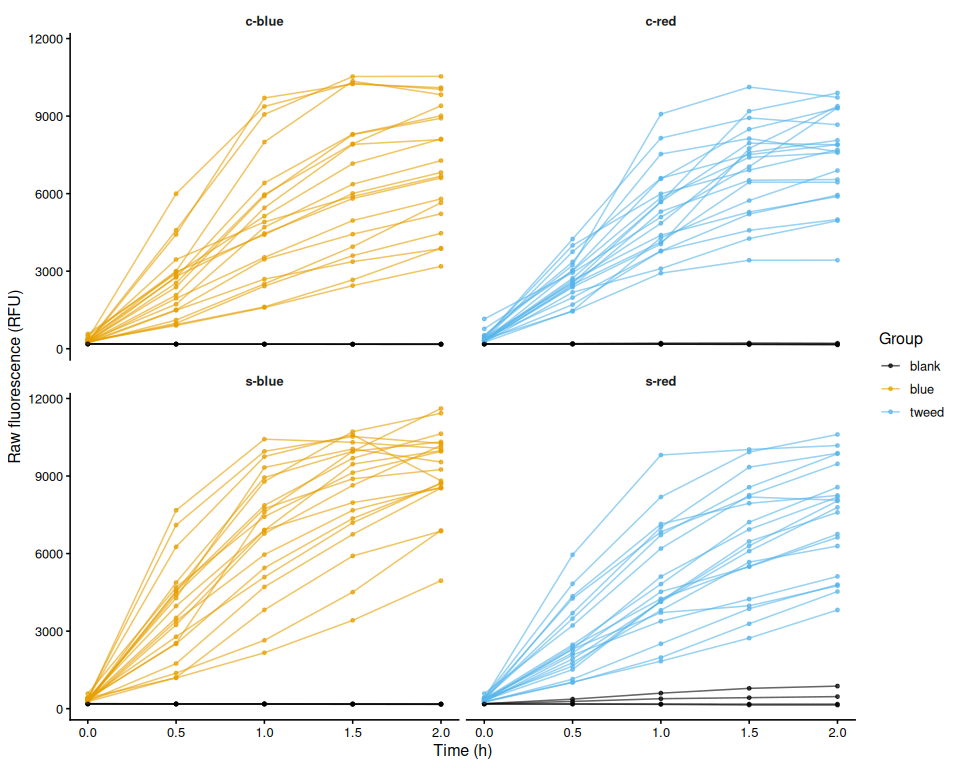

ggsave(file.path(fig_dir, "raw_fluor_by_plate.png"),
       p_raw_plates, width = 10, height = 8)

6.3 Mean raw fluorescence by family

raw_family_summary <- raw_df %>%
  group_by(family_id_group, treatment_group, time_hr) %>%
  summarise(
    mean_fluor = mean(value, na.rm = TRUE),
    se_fluor   = sd(value, na.rm = TRUE) /
      sqrt(sum(!is.na(value))),
    n          = sum(!is.na(value)),
    .groups    = "drop"
  )

p_raw_mean <- ggplot(raw_family_summary,
    aes(x = time_hr, y = mean_fluor,
        color = family_id_group, linetype = treatment_group,
        group = interaction(family_id_group, treatment_group))) +
  geom_ribbon(aes(ymin = mean_fluor - se_fluor,
                  ymax = mean_fluor + se_fluor,
                  fill = family_id_group),
              alpha = 0.15, color = NA) +
  geom_line(linewidth = 1) +
  geom_point(size = 2) +
  scale_color_manual(values = fam_colors, name = "Family") +
  scale_fill_manual(values = fam_colors, name = "Family") +
  scale_linetype_manual(values = trt_linetypes, name = "Treatment") +
  labs(x = "Time (h)", y = "Mean raw fluorescence (RFU ± SE)") +
  theme_classic(base_size = 13)

p_raw_mean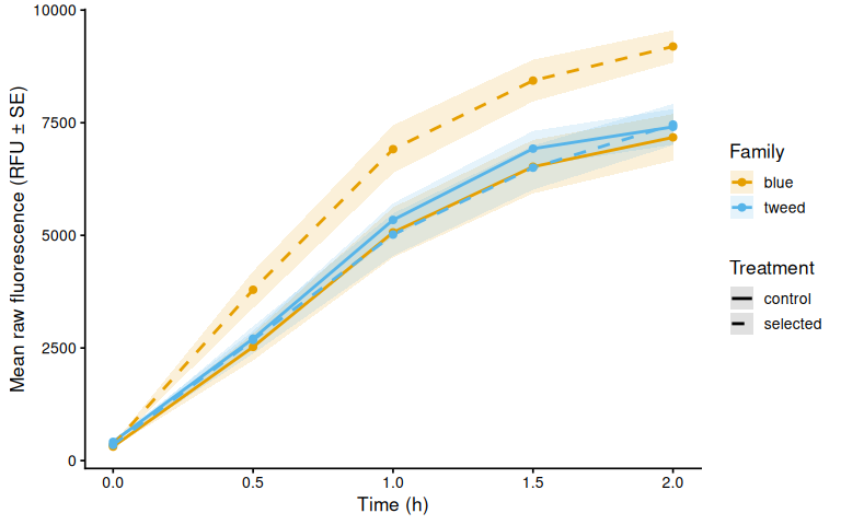

ggsave(file.path(fig_dir, "raw_mean_by_family.png"),
       p_raw_mean, width = 8, height = 5)

6.4 Individual raw fluorescence traces by family

p_raw_by_family <- raw_df %>%
  ggplot(aes(x = time_hr, y = value,
             group = trace_id, color = treatment_group)) +
  geom_line(alpha = 0.6) +
  geom_point(size = 1.2, alpha = 0.7) +
  facet_wrap(~ family_id_group) +
  scale_color_manual(values = trt_colors, name = "Treatment") +
  labs(x = "Time (h)", y = "Raw fluorescence (RFU)") +
  theme_classic(base_size = 12) +
  theme(strip.background = element_blank(),
        strip.text       = element_text(face = "bold"))

p_raw_by_family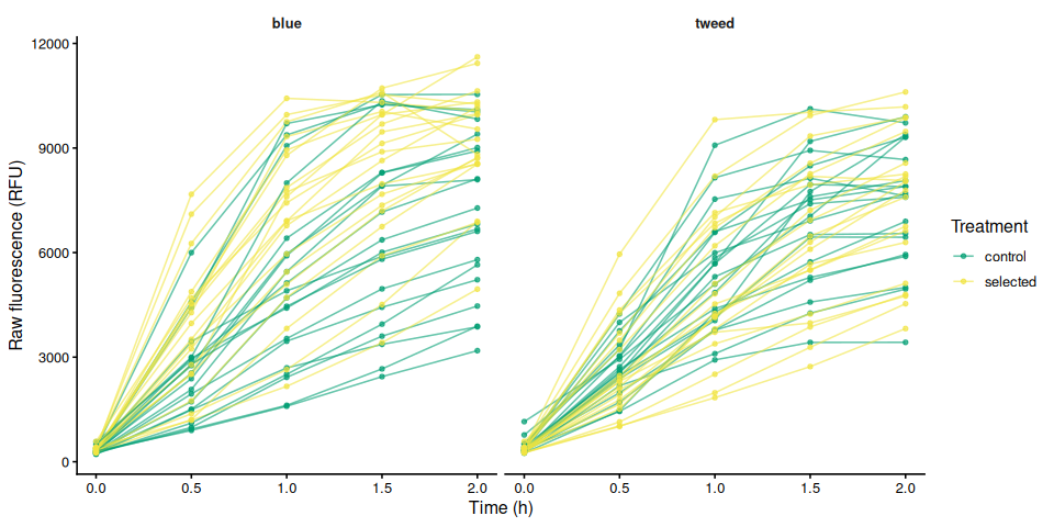

ggsave(file.path(fig_dir, "raw_individual_by_family.png"),
       p_raw_by_family, width = 10, height = 5)

6.5 Individual raw fluorescence traces by treatment

p_raw_by_treatment <- raw_df %>%
  ggplot(aes(x = time_hr, y = value,
             group = trace_id, color = family_id_group)) +
  geom_line(alpha = 0.6) +
  geom_point(size = 1.2, alpha = 0.7) +
  facet_wrap(~ treatment_group) +
  scale_color_manual(values = fam_colors, name = "Family") +
  labs(x = "Time (h)", y = "Raw fluorescence (RFU)") +
  theme_classic(base_size = 12) +
  theme(strip.background = element_blank(),
        strip.text       = element_text(face = "bold"))

p_raw_by_treatment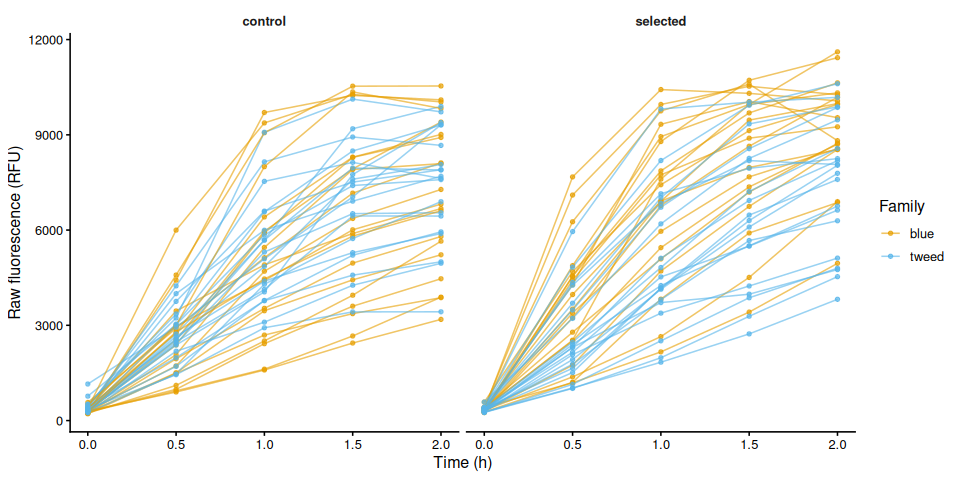

ggsave(file.path(fig_dir, "raw_individual_by_treatment.png"),
       p_raw_by_treatment, width = 10, height = 5)

6.6 Excluded samples

Wells flagged exclude_from_analysis = TRUE appear in the raw fluorescence plots above but are omitted from all analyses that follow.

excluded_wells <- dat %>%
  filter(!is_blank, exclude_from_analysis) %>%
  mutate(
    sample = if_else(
      !is.na(sample_id_group) & trimws(as.character(sample_id_group)) != "",
      as.character(sample_id_group),
      paste(plate_id, well_id, sep = "_")
    )
  ) %>%
  select(plate_id, well_id, sample, family_id_group, treatment_group,
         any_of("exclude_reason")) %>%
  distinct() %>%
  arrange(plate_id, well_id)

if (nrow(excluded_wells) > 0) {
  col_names <- c("Plate", "Well", "Sample", "Family", "Treatment")
  if ("exclude_reason" %in% names(excluded_wells))
    col_names <- c(col_names, "Reason")
  cat(knitr::kable(excluded_wells, col.names = col_names), sep = "\n")
} else {
  cat("No wells are excluded from analysis.\n")
}

No wells are excluded from analysis.

7 Blank Correction via Fold-Change Normalization

Following Huffmyer et al.: fluorescence is first expressed as fold-change relative to each well’s own T0 reading (applied to samples and blanks alike), the mean fold-change of blank wells (per plate, per timepoint) is then subtracted. All samples therefore start at exactly 0 at T0 by construction, eliminating the risk of negative starting values from pipetting variance.

7.1 Step 1 – Fold-change relative to T0 for all wells

t0_all <- dat %>%
  filter(is.finite(time_hr), is.finite(value)) %>%
  group_by(plate_id, well_id) %>%
  slice_min(time_hr, n = 1, with_ties = FALSE) %>%
  select(plate_id, well_id, value_t0 = value) %>%
  ungroup()

dat_fc <- dat %>%
  left_join(t0_all, by = c("plate_id", "well_id")) %>%
  mutate(fold_change = if_else(
    is.finite(value_t0) & value_t0 > 0,
    value / value_t0,
    NA_real_
  ))

str(dat_fc)

tibble [480 × 18] (S3: tbl_df/tbl/data.frame)
 $ row_id               : chr [1:480] "A" "A" "A" "A" ...
 $ col_id               : int [1:480] 1 2 3 4 5 6 1 2 3 4 ...
 $ well_id              : chr [1:480] "A1" "A2" "A3" "A4" ...
 $ value                : num [1:480] 230 304 253 376 389 184 278 493 233 302 ...
 $ plate_id             : chr [1:480] "c-blue" "c-blue" "c-blue" "c-blue" ...
 $ time_hr              : num [1:480] 0 0 0 0 0 0 0 0 0 0 ...
 $ is_blank             : logi [1:480] FALSE FALSE FALSE FALSE FALSE TRUE ...
 $ exclude_from_analysis: logi [1:480] FALSE FALSE FALSE FALSE FALSE FALSE ...
 $ exclude_reason       : chr [1:480] NA NA NA NA ...
 $ family_id_group      : chr [1:480] "blue" "blue" "blue" "blue" ...
 $ sample_id_group      : chr [1:480] "1" "2" "3" "4" ...
 $ treatment_group      : chr [1:480] "control" "control" "control" "control" ...
 $ width_mm_measurement : num [1:480] NA NA NA NA NA NA NA NA NA NA ...
 $ length_mm_measurement: num [1:480] NA NA NA NA NA NA NA NA NA NA ...
 $ weight_mg_measurement: num [1:480] NA NA NA NA NA NA NA NA NA NA ...
 $ area_mm2_measurement : num [1:480] 104.7 102.2 84.6 59.2 86.1 ...
 $ value_t0             : num [1:480] 230 304 253 376 389 184 278 493 233 302 ...
 $ fold_change          : num [1:480] 1 1 1 1 1 1 1 1 1 1 ...

7.2 Step 2 – Mean blank fold-change per plate per timepoint

blank_fc_ref <- dat_fc %>%
  filter(is_blank) %>%
  group_by(plate_id, time_hr) %>%
  summarise(mean_blank_fc = mean(fold_change, na.rm = TRUE),
            .groups = "drop")

str(blank_fc_ref)

tibble [20 × 3] (S3: tbl_df/tbl/data.frame)
 $ plate_id     : chr [1:20] "c-blue" "c-blue" "c-blue" "c-blue" ...
 $ time_hr      : num [1:20] 0 0.5 1 1.5 2 0 0.5 1 1.5 2 ...
 $ mean_blank_fc: num [1:20] 1 0.965 0.956 0.941 0.945 ...

7.3 Step 3 – Subtract blank fold-change from sample fold-change

samples <- dat_fc %>%
  filter(!is_blank, !exclude_from_analysis) %>%
  mutate(
    trace_id = if_else(
      !is.na(sample_id_group) & trimws(as.character(sample_id_group)) != "",
      as.character(sample_id_group),
      paste(plate_id, well_id, sep = "_")
    )
  ) %>%
  left_join(blank_fc_ref, by = c("plate_id", "time_hr")) %>%
  mutate(corrected_fc = fold_change - mean_blank_fc)

str(samples)

tibble [400 × 21] (S3: tbl_df/tbl/data.frame)
 $ row_id               : chr [1:400] "A" "A" "A" "A" ...
 $ col_id               : int [1:400] 1 2 3 4 5 1 2 3 4 5 ...
 $ well_id              : chr [1:400] "A1" "A2" "A3" "A4" ...
 $ value                : num [1:400] 230 304 253 376 389 278 493 233 302 232 ...
 $ plate_id             : chr [1:400] "c-blue" "c-blue" "c-blue" "c-blue" ...
 $ time_hr              : num [1:400] 0 0 0 0 0 0 0 0 0 0 ...
 $ is_blank             : logi [1:400] FALSE FALSE FALSE FALSE FALSE FALSE ...
 $ exclude_from_analysis: logi [1:400] FALSE FALSE FALSE FALSE FALSE FALSE ...
 $ exclude_reason       : chr [1:400] NA NA NA NA ...
 $ family_id_group      : chr [1:400] "blue" "blue" "blue" "blue" ...
 $ sample_id_group      : chr [1:400] "1" "2" "3" "4" ...
 $ treatment_group      : chr [1:400] "control" "control" "control" "control" ...
 $ width_mm_measurement : num [1:400] NA NA NA NA NA NA NA NA NA NA ...
 $ length_mm_measurement: num [1:400] NA NA NA NA NA NA NA NA NA NA ...
 $ weight_mg_measurement: num [1:400] NA NA NA NA NA NA NA NA NA NA ...
 $ area_mm2_measurement : num [1:400] 104.7 102.2 84.6 59.2 86.1 ...
 $ value_t0             : num [1:400] 230 304 253 376 389 278 493 233 302 232 ...
 $ fold_change          : num [1:400] 1 1 1 1 1 1 1 1 1 1 ...
 $ trace_id             : chr [1:400] "1" "2" "3" "4" ...
 $ mean_blank_fc        : num [1:400] 1 1 1 1 1 1 1 1 1 1 ...
 $ corrected_fc         : num [1:400] 0 0 0 0 0 0 0 0 0 0 ...

8 Blank-Corrected Fold-Change

8.1 Mean by family

bc_fc_summary <- samples %>%
  group_by(family_id_group, treatment_group, time_hr) %>%
  summarise(
    mean_val = mean(corrected_fc, na.rm = TRUE),
    se_val   = sd(corrected_fc, na.rm = TRUE) /
      sqrt(sum(!is.na(corrected_fc))),
    n        = sum(!is.na(corrected_fc)),
    .groups  = "drop"
  )

p_bc_fc_mean <- ggplot(bc_fc_summary,
    aes(x = time_hr, y = mean_val,
        color = family_id_group, linetype = treatment_group,
        group = interaction(family_id_group, treatment_group))) +
  geom_ribbon(aes(ymin = mean_val - se_val,
                  ymax = mean_val + se_val,
                  fill = family_id_group),
              alpha = 0.15, color = NA) +
  geom_line(linewidth = 1) +
  geom_point(size = 2) +
  scale_color_manual(values = fam_colors, name = "Family") +
  scale_fill_manual(values = fam_colors, name = "Family") +
  scale_linetype_manual(values = trt_linetypes, name = "Treatment") +
  labs(x = "Time (h)",
       y = "Mean blank-corrected fold-change (± SE)") +
  theme_classic(base_size = 13)

p_bc_fc_mean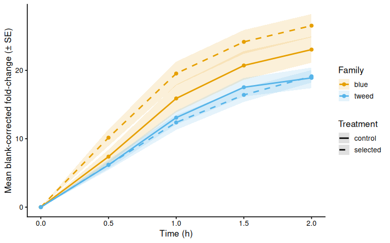

ggsave(file.path(fig_dir, "blank_corrected_fc_mean_by_family.png"),
       p_bc_fc_mean, width = 8, height = 5)

8.2 Individual traces by family

p_bc_fc_by_family <- samples %>%
  ggplot(aes(x = time_hr, y = corrected_fc,
             group = trace_id, color = treatment_group)) +
  geom_line(alpha = 0.6) +
  geom_point(size = 1.2, alpha = 0.7) +
  facet_wrap(~ family_id_group) +
  scale_color_manual(values = trt_colors, name = "Treatment") +
  labs(x = "Time (h)", y = "Blank-corrected fold-change") +
  theme_classic(base_size = 12) +
  theme(strip.background = element_blank(),
        strip.text       = element_text(face = "bold"))

p_bc_fc_by_family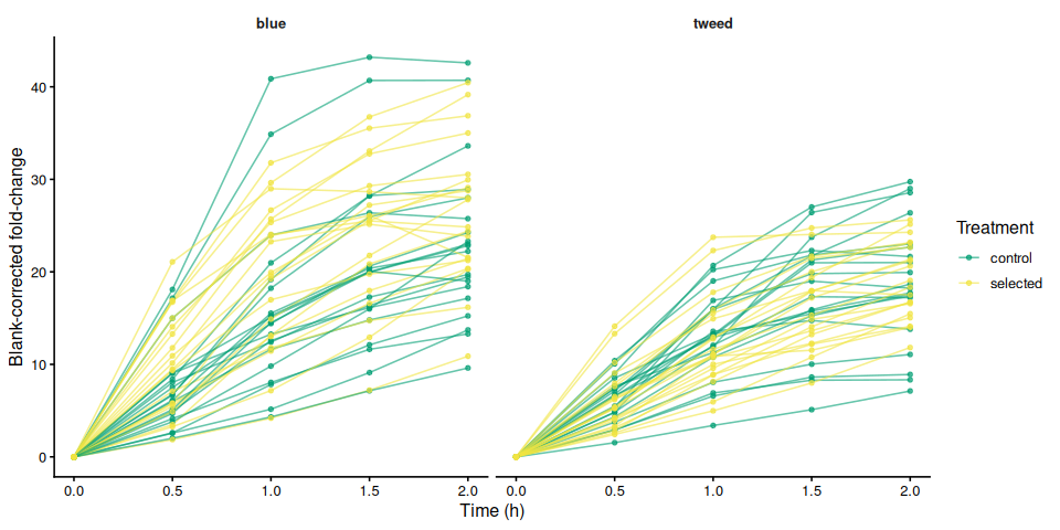

ggsave(file.path(fig_dir, "blank_corrected_fc_by_family.png"),
       p_bc_fc_by_family, width = 10, height = 5)

8.3 Individual blank-corrected fold-change traces by treatment

p_bc_fc_by_treatment <- samples %>%
  ggplot(aes(x = time_hr, y = corrected_fc,
             group = trace_id, color = family_id_group)) +
  geom_line(alpha = 0.6) +
  geom_point(size = 1.2, alpha = 0.7) +
  facet_wrap(~ treatment_group) +
  scale_color_manual(values = fam_colors, name = "Family") +
  labs(x = "Time (h)", y = "Blank-corrected fold-change") +
  theme_classic(base_size = 12) +
  theme(strip.background = element_blank(),
        strip.text       = element_text(face = "bold"))

p_bc_fc_by_treatment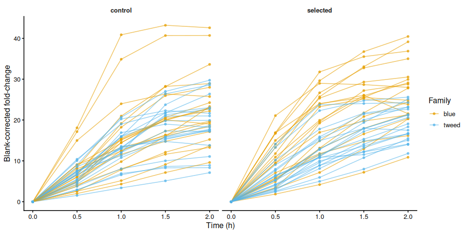

ggsave(file.path(fig_dir, "blank_corrected_fc_by_treatment.png"),
       p_bc_fc_by_treatment, width = 10, height = 5)

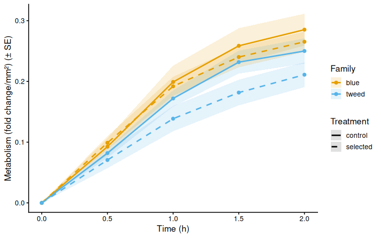
9 Metabolism (Size-Normalised Fold-Change)

Blank-corrected fold-change divided by each active measurement column. This is “metabolism” as defined in Huffmyer et al.

if (length(active_meas_cols) == 0) {
  message("No active measurement columns: skipping metabolism calculation.")
  metabolism_df <- tibble()
} else {
  metabolism_df <- samples
  for (mc in active_meas_cols) {
    out_col <- paste0("metabolism_per_", mc)
    metabolism_df <- metabolism_df %>%
      mutate(!!out_col := if_else(
        is.finite(.data[[mc]]) & .data[[mc]] > 0 &
          is.finite(corrected_fc),
        corrected_fc / .data[[mc]],
        NA_real_
      ))
  }
}

str(metabolism_df)

tibble [400 × 22] (S3: tbl_df/tbl/data.frame)
 $ row_id                             : chr [1:400] "A" "A" "A" "A" ...
 $ col_id                             : int [1:400] 1 2 3 4 5 1 2 3 4 5 ...
 $ well_id                            : chr [1:400] "A1" "A2" "A3" "A4" ...
 $ value                              : num [1:400] 230 304 253 376 389 278 493 233 302 232 ...
 $ plate_id                           : chr [1:400] "c-blue" "c-blue" "c-blue" "c-blue" ...
 $ time_hr                            : num [1:400] 0 0 0 0 0 0 0 0 0 0 ...
 $ is_blank                           : logi [1:400] FALSE FALSE FALSE FALSE FALSE FALSE ...
 $ exclude_from_analysis              : logi [1:400] FALSE FALSE FALSE FALSE FALSE FALSE ...
 $ exclude_reason                     : chr [1:400] NA NA NA NA ...
 $ family_id_group                    : chr [1:400] "blue" "blue" "blue" "blue" ...
 $ sample_id_group                    : chr [1:400] "1" "2" "3" "4" ...
 $ treatment_group                    : chr [1:400] "control" "control" "control" "control" ...
 $ width_mm_measurement               : num [1:400] NA NA NA NA NA NA NA NA NA NA ...
 $ length_mm_measurement              : num [1:400] NA NA NA NA NA NA NA NA NA NA ...
 $ weight_mg_measurement              : num [1:400] NA NA NA NA NA NA NA NA NA NA ...
 $ area_mm2_measurement               : num [1:400] 104.7 102.2 84.6 59.2 86.1 ...
 $ value_t0                           : num [1:400] 230 304 253 376 389 278 493 233 302 232 ...
 $ fold_change                        : num [1:400] 1 1 1 1 1 1 1 1 1 1 ...
 $ trace_id                           : chr [1:400] "1" "2" "3" "4" ...
 $ mean_blank_fc                      : num [1:400] 1 1 1 1 1 1 1 1 1 1 ...
 $ corrected_fc                       : num [1:400] 0 0 0 0 0 0 0 0 0 0 ...
 $ metabolism_per_area_mm2_measurement: num [1:400] 0 0 0 0 0 0 0 0 0 0 ...

9.1 Mean metabolism by family

if (nrow(metabolism_df) > 0) {

  metab_cols <- paste0("metabolism_per_", active_meas_cols)

  for (col in metab_cols) {
    if (!col %in% names(metabolism_df)) next
    mc_label <- str_remove(col, "^metabolism_per_")

    metab_summary <- metabolism_df %>%
      group_by(family_id_group, treatment_group, time_hr) %>%
      summarise(
        mean_val = mean(.data[[col]], na.rm = TRUE),
        se_val   = sd(.data[[col]], na.rm = TRUE) /
          sqrt(sum(!is.na(.data[[col]]))),
        .groups  = "drop"
      )

    p_metab_mean <- ggplot(metab_summary,
        aes(x = time_hr, y = mean_val,
            color = family_id_group, linetype = treatment_group,
            group = interaction(family_id_group, treatment_group))) +
      geom_ribbon(aes(ymin = mean_val - se_val,
                      ymax = mean_val + se_val,
                      fill = family_id_group),
                  alpha = 0.15, color = NA) +
      geom_line(linewidth = 1) +
      geom_point(size = 2) +
      scale_color_manual(values = fam_colors, name = "Family") +
      scale_fill_manual(values = fam_colors, name = "Family") +
      scale_linetype_manual(values = trt_linetypes, name = "Treatment") +
      labs(x = "Time (h)",
           y = paste0(metabolism_y_label(col), " (± SE)")) +
      theme_classic(base_size = 13)

    print(p_metab_mean)
    ggsave(
      file.path(fig_dir,
                paste0("metabolism_mean_", mc_label, ".png")),
      p_metab_mean, width = 8, height = 5)
  }
}

9.2 Individual metabolism traces by family

if (nrow(metabolism_df) > 0) {

  for (col in metab_cols) {
    if (!col %in% names(metabolism_df)) next
    mc_label <- str_remove(col, "^metabolism_per_")

    p_metab_by_family <- ggplot(metabolism_df,
        aes(x = time_hr, y = .data[[col]],
            group = trace_id, color = treatment_group)) +
      geom_line(alpha = 0.6) +
      geom_point(size = 1.2, alpha = 0.7) +
      facet_wrap(~ family_id_group) +
      scale_color_manual(values = trt_colors, name = "Treatment") +
      labs(x = "Time (h)", y = metabolism_y_label(col)) +
      theme_classic(base_size = 12) +
      theme(strip.background = element_blank(),
            strip.text       = element_text(face = "bold"))

    print(p_metab_by_family)
    ggsave(
      file.path(fig_dir,
                paste0("metabolism_individual_", mc_label, "_by_family.png")),
      p_metab_by_family, width = 10, height = 5)

    p_metab_by_treatment <- ggplot(metabolism_df,
        aes(x = time_hr, y = .data[[col]],
            group = trace_id, color = family_id_group)) +
      geom_line(alpha = 0.6) +
      geom_point(size = 1.2, alpha = 0.7) +
      facet_wrap(~ treatment_group) +
      scale_color_manual(values = fam_colors, name = "Family") +
      labs(x = "Time (h)", y = metabolism_y_label(col)) +
      theme_classic(base_size = 12) +
      theme(strip.background = element_blank(),
            strip.text       = element_text(face = "bold"))

    print(p_metab_by_treatment)
    ggsave(
      file.path(fig_dir,
                paste0("metabolism_individual_", mc_label, "_by_treatment.png")),
      p_metab_by_treatment, width = 10, height = 5)
  }
}

10 Time-Series Statistical Analysis

Linear mixed effects models test the effect of experimental variables on metabolism over time. Individual (sample_id_group) is included as a random intercept to account for repeated measures across timepoints. Type III ANOVA with Satterthwaite’s approximation (lmerTest) assesses significance; post-hoc pairwise comparisons use estimated marginal means (emmeans, Tukey adjustment).

run_ts_stats <- function(df, value_col) {
  has_family    <- "family_id_group" %in% names(df) &&
    length(unique(na.omit(df$family_id_group))) > 1
  has_treatment <- "treatment_group" %in% names(df) &&
    length(unique(na.omit(df$treatment_group))) > 1

  if (!has_family && !has_treatment) return(NULL)

  df <- df %>%
    filter(is.finite(.data[[value_col]]), is.finite(time_hr)) %>%
    mutate(
      time_f     = factor(time_hr),
      individual = factor(trace_id)
    )

  if (nrow(df) == 0) return(NULL)

  if (has_family)    df <- df %>% mutate(family    = factor(family_id_group))
  if (has_treatment) df <- df %>% mutate(treatment = factor(treatment_group))

  if (has_family    && length(unique(na.omit(df$family)))    < 2) return(NULL)
  if (has_treatment && length(unique(na.omit(df$treatment))) < 2) return(NULL)

  fixed <- if (has_family && has_treatment)
    paste0(value_col, " ~ time_f * family * treatment")
  else if (has_family)
    paste0(value_col, " ~ time_f * family")
  else
    paste0(value_col, " ~ time_f * treatment")

  model <- lmer(
    as.formula(paste0(fixed, " + (1 | individual)")),
    data = df
  )

  anova_res <- anova(model, type = 3, ddf = "Satterthwaite")

  # Pairwise comparisons of group combinations at each timepoint
  emm_spec <- if (has_family && has_treatment)
    ~ family * treatment | time_f
  else if (has_family)
    ~ family | time_f
  else
    ~ treatment | time_f

  emm       <- emmeans(model, emm_spec)
  pairs_res <- as.data.frame(pairs(emm, adjust = "tukey"))

  # Main-effect marginal means (collapsed across time)
  emm_main <- if (has_family && has_treatment)
    emmeans(model, ~ family * treatment)
  else if (has_family)
    emmeans(model, ~ family)
  else
    emmeans(model, ~ treatment)

  pairs_main <- as.data.frame(pairs(emm_main, adjust = "tukey"))

  list(
    model         = model,
    anova         = anova_res,
    pairs_by_time = pairs_res,
    pairs_main    = pairs_main,
    has_family    = has_family,
    has_treatment = has_treatment
  )
}

ts_stats <- list()
if (nrow(metabolism_df) > 0) {
  for (mc in active_meas_cols) {
    col <- paste0("metabolism_per_", mc)
    if (col %in% names(metabolism_df))
      ts_stats[[col]] <- run_ts_stats(metabolism_df, col)
  }
}

10.1 Results

for (col in names(ts_stats)) {
  res <- ts_stats[[col]]
  if (is.null(res)) next

  cat("\n\n----\n### Metric:", col, "\n\n")

  cat("**Type III ANOVA (Satterthwaite approximation):**\n")
  print(res$anova)

  cat("\n**Marginal means – main effects (collapsed across time):**\n")
  print(res$pairs_main)

  cat("\n**Pairwise comparisons by timepoint (Tukey):**\n")
  print(res$pairs_by_time)
}

### Metric: metabolism_per_area_mm2_measurement
Signif. codes: 0 ‘’ 0.001 ’’ 0.01 ’’ 0.05 ‘.’ 0.1 ’ ’ 1
Marginal means – main effects (collapsed across time): contrast estimate SE df t.ratio p.value blue control - tweed control 0.01994712 0.02039961 76 0.978 0.7625 blue control - blue selected 0.00783381 0.02039961 76 0.384 0.9806 blue control - tweed selected 0.04671200 0.02039961 76 2.290 0.1095 tweed control - blue selected -0.01211331 0.02039961 76 -0.594 0.9337 tweed control - tweed selected 0.02676488 0.02039961 76 1.312 0.5582 blue selected - tweed selected 0.03887819 0.02039961 76 1.906 0.2343
Results are averaged over the levels of: time_f Degrees-of-freedom method: kenward-roger P value adjustment: tukey method for comparing a family of 4 estimates
Pairwise comparisons by timepoint (Tukey): time_f = 0: contrast estimate SE df t.ratio p.value blue control - tweed control 0.00000000 0.02424006 145.35 0.000 1.0000 blue control - blue selected 0.00000000 0.02424006 145.35 0.000 1.0000 blue control - tweed selected 0.00000000 0.02424006 145.35 0.000 1.0000 tweed control - blue selected 0.00000000 0.02424006 145.35 0.000 1.0000 tweed control - tweed selected 0.00000000 0.02424006 145.35 0.000 1.0000 blue selected - tweed selected 0.00000000 0.02424006 145.35 0.000 1.0000
time_f = 0.5: contrast estimate SE df t.ratio p.value blue control - tweed control 0.01058815 0.02424006 145.35 0.437 0.9720 blue control - blue selected -0.00633532 0.02424006 145.35 -0.261 0.9937 blue control - tweed selected 0.02197331 0.02424006 145.35 0.906 0.8014 tweed control - blue selected -0.01692347 0.02424006 145.35 -0.698 0.8976 tweed control - tweed selected 0.01138517 0.02424006 145.35 0.470 0.9656 blue selected - tweed selected 0.02830864 0.02424006 145.35 1.168 0.6481
time_f = 1: contrast estimate SE df t.ratio p.value blue control - tweed control 0.02713104 0.02424006 145.35 1.119 0.6783 blue control - blue selected 0.00712265 0.02424006 145.35 0.294 0.9911 blue control - tweed selected 0.06043328 0.02424006 145.35 2.493 0.0652 tweed control - blue selected -0.02000840 0.02424006 145.35 -0.825 0.8423 tweed control - tweed selected 0.03330224 0.02424006 145.35 1.374 0.5178 blue selected - tweed selected 0.05331063 0.02424006 145.35 2.199 0.1283
time_f = 1.5: contrast estimate SE df t.ratio p.value blue control - tweed control 0.02687676 0.02424006 145.35 1.109 0.6847 blue control - blue selected 0.01848720 0.02424006 145.35 0.763 0.8711 blue control - tweed selected 0.07696626 0.02424006 145.35 3.175 0.0098 tweed control - blue selected -0.00838956 0.02424006 145.35 -0.346 0.9857 tweed control - tweed selected 0.05008949 0.02424006 145.35 2.066 0.1691 blue selected - tweed selected 0.05847905 0.02424006 145.35 2.412 0.0792
time_f = 2: contrast estimate SE df t.ratio p.value blue control - tweed control 0.03513966 0.02424006 145.35 1.450 0.4707 blue control - blue selected 0.01989453 0.02424006 145.35 0.821 0.8446 blue control - tweed selected 0.07418715 0.02424006 145.35 3.061 0.0139 tweed control - blue selected -0.01524513 0.02424006 145.35 -0.629 0.9226 tweed control - tweed selected 0.03904749 0.02424006 145.35 1.611 0.3757 blue selected - tweed selected 0.05429262 0.02424006 145.35 2.240 0.1175
Degrees-of-freedom method: kenward-roger P value adjustment: tukey method for comparing a family of 4 estimates
# Area Under the Curve (AUC)
AUC computed per individual via the trapezoid rule across all timepoints. metabolism_per_* is the primary metric matching the paper; corrected_fc and raw_fluorescence are retained for reference.
``` r compute_auc <- function(df, value_col, group_vars) { df %>% filter(is.finite(time_hr), is.finite(.data\[\[value_col\]])) %>% group_by(across(all_of(group_vars))) %>% summarise( AUC = trapezoid_auc(time_hr, .data\[\[value_col\]]), n_timepoints = n(), .groups = “drop” ) %>% filter(is.finite(AUC)) }
# Only include grouping columns that are actually present in the data individual_vars <- intersect( c(“trace_id”, “family_id_group”, “treatment_group”), names(metabolism_df) )
auc_metab_list <- list() if (nrow(metabolism_df) > 0) { for (mc in active_meas_cols) { col <- paste0(“metabolism_per_”, mc) if (col %in% names(metabolism_df)) { auc_metab_list\[\[col\]] <- compute_auc(metabolism_df, col, individual_vars) %>% mutate(metric = col) } } }
auc_all <- bind_rows(auc_metab_list)
str(auc_all) ```
tibble [80 × 6] (S3: tbl_df/tbl/data.frame) $ trace_id : chr [1:80] "1" "10" "11" "12" ... $ family_id_group: chr [1:80] "blue" "blue" "blue" "blue" ... $ treatment_group: chr [1:80] "control" "control" "control" "control" ... $ AUC : num [1:80] 0.261 0.722 0.371 0.157 0.143 ... $ n_timepoints : int [1:80] 5 5 5 5 5 5 5 5 5 5 ... $ metric : chr [1:80] "metabolism_per_area_mm2_measurement" "metabolism_per_area_mm2_measurement" "metabolism_per_area_mm2_measurement" "metabolism_per_area_mm2_measurement" ...
## AUC summary tables
``` r sum_vars <- intersect( c(“metric”, “family_id_group”, “treatment_group”), names(auc_all) ) auc_summary <- auc_all %>% group_by(across(all_of(sum_vars))) %>% summarise( n = n(), mean = mean(AUC, na.rm = TRUE), sd = sd(AUC, na.rm = TRUE), se = sd / sqrt(n), median = median(AUC, na.rm = TRUE), .groups = “drop” )
print(auc_summary) ```
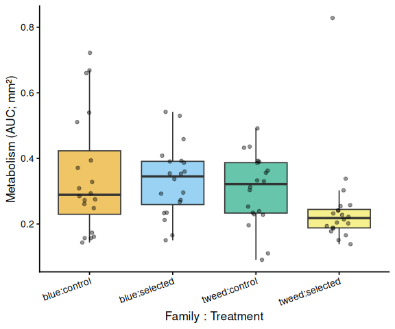
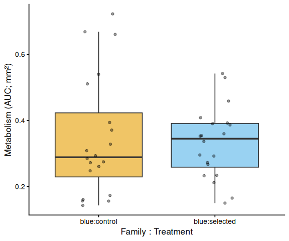
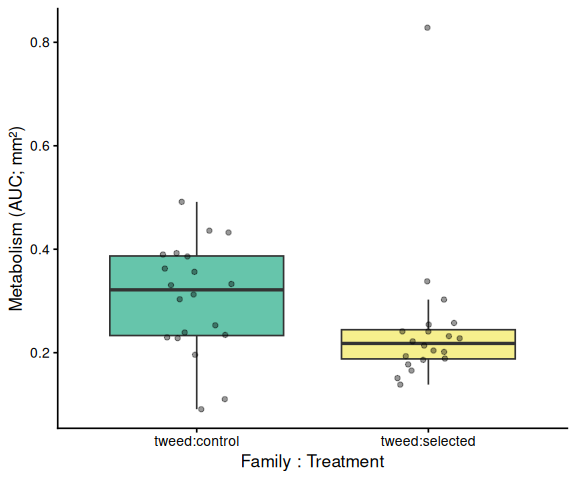
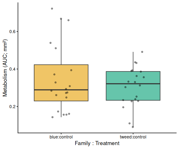
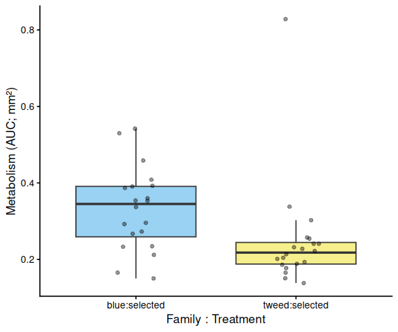
# A tibble: 4 × 8 metric family_id_group treatment_group n mean sd se median <chr> <chr> <chr> <int> <dbl> <dbl> <dbl> <dbl> 1 metabolism_pe… blue control 20 0.346 0.181 0.0405 0.289 2 metabolism_pe… blue selected 20 0.332 0.108 0.0242 0.345 3 metabolism_pe… tweed control 20 0.305 0.107 0.0239 0.322 4 metabolism_pe… tweed selected 20 0.248 0.145 0.0324 0.218
# Statistical Analysis
Each individual clam (sample_id_group) is the observational unit. The model is built from whichever grouping factors are present: both family and treatment (with interaction) when both exist, or a one-way model when only one factor is available. Each plate maps to a unique family × treatment combination, so plate-level and group-level variance are confounded; interpret accordingly.
``` r run_auc_stats <- function(auc_df) { empty <- tibble()
has_family <- “family_id_group” %in% names(auc_df) && length(unique(na.omit(auc_df\(family_id_group))) > 1 has_treatment <- "treatment_group" %in% names(auc_df) && length(unique(na.omit(auc_df\)treatment_group))) > 1
if (!has_family && !has_treatment) { return(list(model = NULL, anova = NULL, pairs_full = empty, pairs_family = empty, pairs_trt = empty, has_family = FALSE, has_treatment = FALSE)) }
if (has_family) auc_df <- auc_df %>% mutate(family = factor(family_id_group)) if (has_treatment) auc_df <- auc_df %>% mutate(treatment = factor(treatment_group))
formula_str <- if (has_family && has_treatment) “AUC ~ family * treatment” else if (has_family) “AUC ~ family” else “AUC ~ treatment” model <- lm(as.formula(formula_str), data = auc_df) anova_res <- anova(model)
if (has_family && has_treatment) { pairs_full <- as.data.frame(pairs(emmeans(model, ~ family * treatment), adjust = “tukey”)) pairs_family <- as.data.frame(pairs(emmeans(model, ~ family), adjust = “tukey”)) pairs_trt <- as.data.frame(pairs(emmeans(model, ~ treatment), adjust = “tukey”)) } else if (has_family) { pairs_family <- as.data.frame(pairs(emmeans(model, ~ family), adjust = “tukey”)) pairs_full <- pairs_family pairs_trt <- empty } else { pairs_trt <- as.data.frame(pairs(emmeans(model, ~ treatment), adjust = “tukey”)) pairs_full <- pairs_trt pairs_family <- empty }
list( model = model, anova = anova_res, pairs_full = pairs_full, pairs_family = pairs_family, pairs_trt = pairs_trt, has_family = has_family, has_treatment = has_treatment ) }
metrics_to_test <- unique(auc_all$metric) stats_results <- map( set_names(metrics_to_test), ~ run_auc_stats(auc_all %>% filter(metric == .x)) ) ```
## Results by metric

10.1.1 Metric: metabolism_per_area_mm2_measurement

ANOVA: Analysis of Variance Table

Response: AUC Df Sum Sq Mean Sq F value Pr(>F)
family 1 0.07776 0.077757 4.0482 0.04776 * treatment 1 0.02575 0.025748 1.3405 0.25057
family:treatment 1 0.00905 0.009048 0.4711 0.49459
Residuals 76 1.45978 0.019208
— Signif. codes: 0 ‘’ 0.001 ’’ 0.01 ’’ 0.05 ‘.’ 0.1 ’ ’ 1

Pairwise: family × treatment (Tukey): contrast estimate SE df t.ratio p.value blue control - tweed control 0.04108289 0.04382646 76 0.937 0.7849 blue control - blue selected 0.01461090 0.04382646 76 0.333 0.9871 blue control - tweed selected 0.09823321 0.04382646 76 2.241 0.1215 tweed control - blue selected -0.02647200 0.04382646 76 -0.604 0.9305 tweed control - tweed selected 0.05715032 0.04382646 76 1.304 0.5633 blue selected - tweed selected 0.08362232 0.04382646 76 1.908 0.2333

P value adjustment: tukey method for comparing a family of 4 estimates

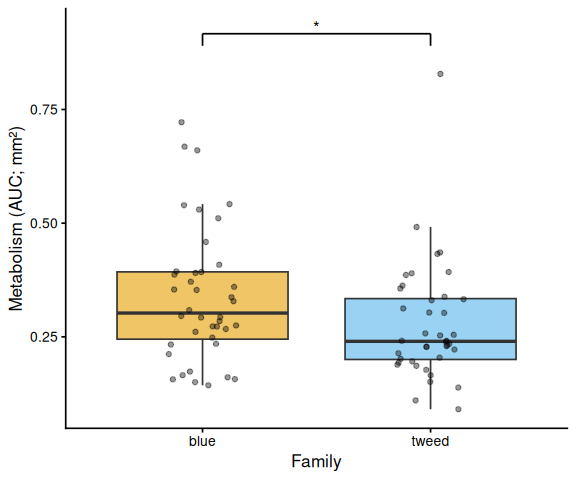
Pairwise: family main effect: contrast estimate SE df t.ratio p.value blue - tweed 0.06235261 0.03098999 76 2.012 0.0478

Results are averaged over the levels of: treatment

Pairwise: treatment main effect: contrast estimate SE df t.ratio p.value control - selected 0.03588061 0.03098999 76 1.158 0.2506

Results are averaged over the levels of: family

11 AUC Box Plots with Statistical Annotations

Significance labels: *** p < 0.001, ** p < 0.01, * p < 0.05. Brackets are drawn only for significant pairs (p < 0.05). Plots are generated for whichever grouping factors are present: treatment-only, family-only, all-groups, within-family, and within-treatment.

sig_label <- function(p) {
  case_when(p < 0.001 ~ "***", p < 0.01 ~ "**", p < 0.05 ~ "*",
            TRUE ~ "ns")
}

# Add significance brackets to an existing ggplot.
# pairs_df   : data frame with $contrast and $p.value columns
# group_levels: ordered character vector matching x-axis factor levels
# y_vals     : numeric vector of AUC values used to set bracket heights
add_sig_brackets <- function(p, pairs_df, group_levels, y_vals) {
  sig_pairs <- pairs_df %>%
    mutate(label = sig_label(p.value)) %>%
    filter(label != "ns")
  if (nrow(sig_pairs) == 0) return(p)

  y_max   <- max(y_vals, na.rm = TRUE)
  y_range <- diff(range(y_vals, na.rm = TRUE))
  step    <- y_range * 0.12

  for (i in seq_len(nrow(sig_pairs))) {
    parts <- str_split(as.character(sig_pairs$contrast[i]), " - ", 2)[[1]]
    g1 <- trimws(parts[1])
    g2 <- trimws(parts[2])
    x1 <- match(g1, group_levels)
    x2 <- match(g2, group_levels)
    if (is.na(x1) || is.na(x2)) next
    bar_y <- y_max + i * step
    p <- p +
      annotate("segment", x = x1, xend = x2,
               y = bar_y, yend = bar_y,
               color = "black", linewidth = 0.6) +
      annotate("segment", x = x1, xend = x1,
               y = bar_y, yend = bar_y - step * 0.3,
               color = "black", linewidth = 0.6) +
      annotate("segment", x = x2, xend = x2,
               y = bar_y, yend = bar_y - step * 0.3,
               color = "black", linewidth = 0.6) +
      annotate("text", x = (x1 + x2) / 2,
               y = bar_y + step * 0.15,
               label = sig_pairs$label[i], size = 4.5)
  }
  p
}

for (met in metrics_to_test) {
  df      <- auc_all %>% filter(metric == met)
  stats   <- stats_results[[met]]
  y_lab   <- auc_y_label(met)
  has_fam <- stats$has_family
  has_trt <- stats$has_treatment

  # ── Treatment main effect (x = treatment, tick = treatment name) ───────
  if (has_trt) {
    df_p <- df %>%
      mutate(x = factor(treatment_group, levels = sort(unique(treatment_group))))
    grps <- levels(df_p$x)
    p <- ggplot(df_p, aes(x = x, y = AUC, fill = x)) +
      geom_boxplot(alpha = 0.6, outlier.shape = NA) +
      geom_jitter(width = 0.15, alpha = 0.4, size = 1.5) +
      scale_fill_manual(values = trt_colors[grps], guide = "none") +
      labs(x = "Treatment", y = y_lab) +
      theme_classic(base_size = 13)
    p <- add_sig_brackets(p, stats$pairs_trt, grps, df_p$AUC)
    print(p)
    ggsave(file.path(fig_dir, paste0("auc_treatment_", met, ".png")),
           p, width = 5, height = 5)
  }

  # ── Family main effect (x = family, tick = family name) ───────────────
  if (has_fam) {
    df_p <- df %>%
      mutate(x = factor(family_id_group, levels = sort(unique(family_id_group))))
    grps <- levels(df_p$x)
    p <- ggplot(df_p, aes(x = x, y = AUC, fill = x)) +
      geom_boxplot(alpha = 0.6, outlier.shape = NA) +
      geom_jitter(width = 0.15, alpha = 0.4, size = 1.5) +
      scale_fill_manual(values = fam_colors[grps], guide = "none") +
      labs(x = "Family", y = y_lab) +
      theme_classic(base_size = 13)
    p <- add_sig_brackets(p, stats$pairs_family, grps, df_p$AUC)
    print(p)
    ggsave(file.path(fig_dir, paste0("auc_family_", met, ".png")),
           p, width = 5, height = 5)
  }

  # Remaining plots require both factors
  if (!has_fam || !has_trt) next

  # ── All family:treatment groups (x = family:treatment) ─────────────────
  # emmeans contrasts use spaces; convert to colon to match tick labels
  pairs_fc <- stats$pairs_full %>%
    mutate(contrast = str_replace_all(
      contrast,
      "([a-z]+) ([a-z]+)( - )([a-z]+) ([a-z]+)",
      "\\1:\\2\\3\\4:\\5"
    ))
  df_p <- df %>%
    mutate(x = factor(
      paste(family_id_group, treatment_group, sep = ":"),
      levels = sort(unique(paste(family_id_group, treatment_group, sep = ":")))
    ))
  grps     <- levels(df_p$x)
  fill_map <- setNames(make_palette(length(grps)), grps)
  p <- ggplot(df_p, aes(x = x, y = AUC, fill = x)) +
    geom_boxplot(alpha = 0.6, outlier.shape = NA) +
    geom_jitter(width = 0.15, alpha = 0.4, size = 1.5) +
    scale_fill_manual(values = fill_map, guide = "none") +
    labs(x = "Family : Treatment", y = y_lab) +
    theme_classic(base_size = 13) +
    theme(axis.text.x = element_text(angle = 20, hjust = 1))
  p <- add_sig_brackets(p, pairs_fc, grps, df_p$AUC)
  print(p)
  ggsave(file.path(fig_dir, paste0("auc_all_groups_", met, ".png")),
         p, width = 6, height = 5)

  # ── Within each family: treatment comparison (x = family:treatment) ────
  # Tick labels are family:treatment so these plots are visually distinct
  # from the treatment main-effect plot above.
  for (fam in sort(unique(df$family_id_group))) {
    df_p <- df %>%
      filter(family_id_group == fam) %>%
      mutate(x = factor(
        paste(family_id_group, treatment_group, sep = ":"),
        levels = sort(unique(paste(family_id_group, treatment_group, sep = ":")))
      ))
    grps     <- levels(df_p$x)
    pairs_sub <- pairs_fc %>%
      filter(str_count(contrast, paste0(fam, ":")) == 2)
    p <- ggplot(df_p, aes(x = x, y = AUC, fill = x)) +
      geom_boxplot(alpha = 0.6, outlier.shape = NA) +
      geom_jitter(width = 0.15, alpha = 0.4, size = 1.5) +
      scale_fill_manual(values = fill_map[grps], guide = "none") +
      labs(x = "Family : Treatment", y = y_lab) +
      theme_classic(base_size = 13)
    p <- add_sig_brackets(p, pairs_sub, grps, df_p$AUC)
    print(p)
    ggsave(file.path(fig_dir, paste0("auc_", fam, "_trt_", met, ".png")),
           p, width = 5, height = 5)
  }

  # ── Within each treatment: family comparison (x = family:treatment) ────
  # Tick labels are family:treatment so these plots are visually distinct
  # from the family main-effect plot above.
  for (trt in sort(unique(df$treatment_group))) {
    df_p <- df %>%
      filter(treatment_group == trt) %>%
      mutate(x = factor(
        paste(family_id_group, treatment_group, sep = ":"),
        levels = sort(unique(paste(family_id_group, treatment_group, sep = ":")))
      ))
    grps      <- levels(df_p$x)
    pairs_sub <- pairs_fc %>%
      filter(str_count(contrast, paste0(":", trt)) == 2)
    p <- ggplot(df_p, aes(x = x, y = AUC, fill = x)) +
      geom_boxplot(alpha = 0.6, outlier.shape = NA) +
      geom_jitter(width = 0.15, alpha = 0.4, size = 1.5) +
      scale_fill_manual(values = fill_map[grps], guide = "none") +
      labs(x = "Family : Treatment", y = y_lab) +
      theme_classic(base_size = 13)
    p <- add_sig_brackets(p, pairs_sub, grps, df_p$AUC)
    print(p)
    ggsave(file.path(fig_dir, paste0("auc_", trt, "_fam_", met, ".png")),
           p, width = 5, height = 5)
  }
}

12 Save Output Data

write_csv(auc_all,      file.path(out_dir, "auc_all_metrics.csv"))
write_csv(auc_summary,  file.path(out_dir, "auc_summary.csv"))

if (nrow(metabolism_df) > 0)
  write_csv(metabolism_df,
            file.path(out_dir, "metabolism.csv"))

stats_compiled <- map_dfr(metrics_to_test, function(met) {
  bind_rows(
    stats_results[[met]]$pairs_full %>%
      mutate(comparison = "family:treatment"),
    stats_results[[met]]$pairs_family %>%
      mutate(comparison = "family"),
    stats_results[[met]]$pairs_trt %>%
      mutate(comparison = "treatment")
  ) %>% mutate(metric = met)
})

write_csv(stats_compiled,
          file.path(out_dir, "pairwise_stats.csv"))

message("Output files written to: ", out_dir)

---

MATERIALS & METHODS

Steven picked 48 clams from the “Selected” group and 48 clams from the “Control” group.

Two plates per treatment were measured: “blue” and “red”. The colors reflect the coloration of the clams.

Blanks were included on each plate, and consisted of wells with resazurin working solution, but no clams. Blanks were in Column 6 of each plate.

Plates were kept in a small, table-top, fan-powered incubator at 40^oC.

Resazurin Working Solution

Clams were processed in 24-well plates and submerged in 2.2mL of resazurin working solution; prepared by Sam White 20260330:

• 986.66 mL filtered seawater (4^oC filtered sea water from 11/19/2025 by AH)
• 2.22 mL resazurin stock solution (from step 1 above)
• 1.00 mL DMSO
• 10.00 mL antibiotic solution (100x Penn/Strep & 100x Fungizone)

Measurements

Plates were measured every 30mins on a Synergy HTX (Agilent) plate reader. The plate reader was set to measure fluorescence with an excitation wavelength of 530nm and an emission wavelength of 590nm.

RESULTS

All four plates passed the consistency check (24 wells per plate at every timepoint), and no individual wells were flagged for exclusion.

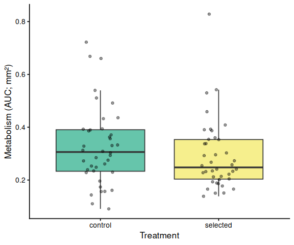
Metabolic activity (AUC of blank-corrected, size-normalised fold-change per mm² shell area) did not differ significantly between selected and control clams (ANOVA: F = 1.34, p = 0.251; Tukey pairwise: control − selected estimate = 0.036, p = 0.251).

Shell-color family was a significant predictor of metabolism (ANOVA: F = 4.05, p = 0.048), with blue-family clams showing higher metabolic activity than tweed-family clams (estimate = 0.062, p = 0.048). No significant family × treatment interaction was detected (p = 0.495).

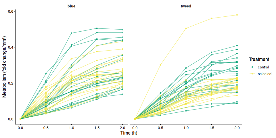
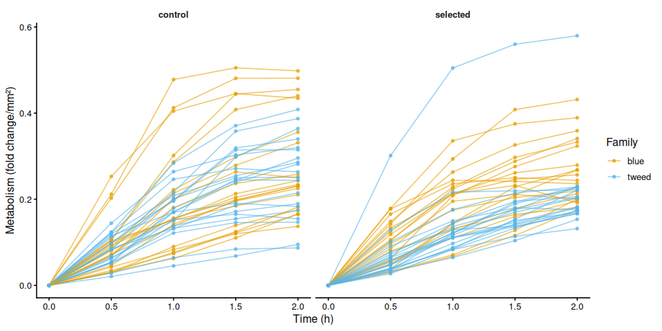
The time-series linear mixed-effects model (metabolism ~ time × family × treatment, random intercept per individual) corroborated these patterns. The only significant pairwise differences at individual timepoints were between blue control and tweed selected clams at 1.5 h (p = 0.010) and 2.0 h (p = 0.014), reflecting the family-level divergence rather than a treatment effect.

In summary, there was no evidence that selected clams have higher metabolic activity than control clams under 40°C acute heat stress in this assay. The primary source of metabolic variation was shell-color family identity.