We carried out whole genome BS-Seq on siblings outplanted out at two sites: Fidalgo Bay (home) and Oyster Bay. Four individuals from each locale were examined.
A running description of the data is available @ https://github.com/RobertsLab/project-olympia.oyster-genomic/wiki/Whole-genome-BSseq-December-2015.
I need to look back to a genome to analyze this. We did some PacBio sequencing a while ago.
– http://nbviewer.jupyter.org/github/sr320/ipython_nb/blob/master/OlyO_PacBio.ipynb
In recap, the fastq file had 47,475 reads: http://owl.fish.washington.edu/halfshell/OlyO_Pat_PacBio_1.fastq
3058 of these reads were >10k bp: http://eagle.fish.washington.edu/cnidarian/OlyO_Pat_PacBio_10k.fa
Those 3058 reads were nicely assembled into 553 contigs: http://eagle.fish.washington.edu/cnidarian/OlyO_Pat_PacBio_10k_contigs.fa
Step forward a bit and all 47475 reads were assembled into the 5362 contigs known as OlyO_Pat_v02.fa http://owl.fish.washington.edu/halfshell/OlyO_Pat_v02.fa
The latter (v02) was used to map the 8 libraries. Roughly getting about 8% mapping
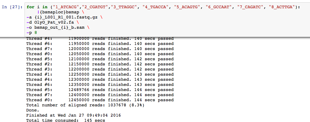
About 15 fold average coverage

And with a little filtering
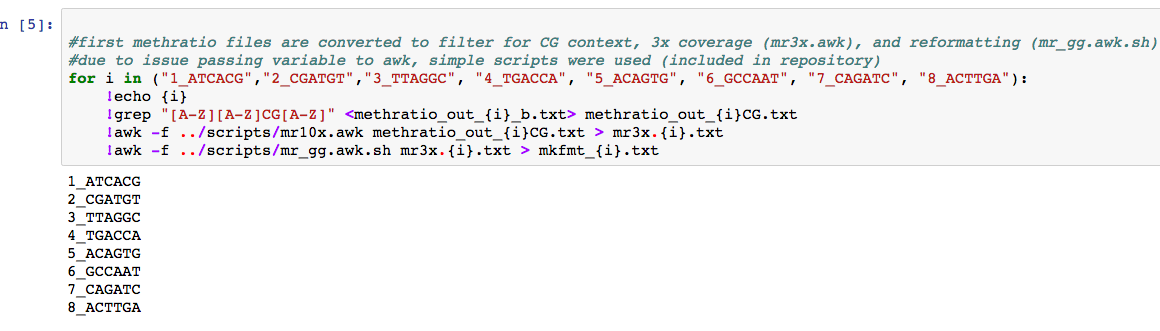
Note that awk script filtered for 10x coverage! this could be altered.
and R have an intriguing relationship

With BGI Draft Genome
Following the same workflow with the BGIv1 scaffolds >10k bp have about 16% or reads map.
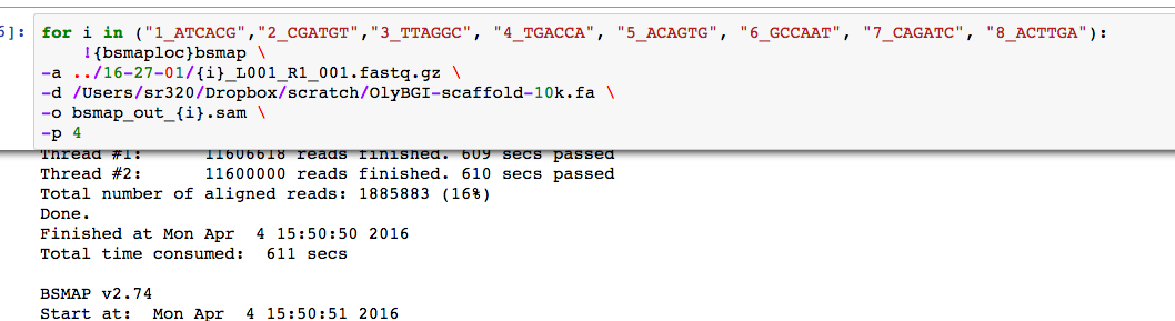
3 fold coverage
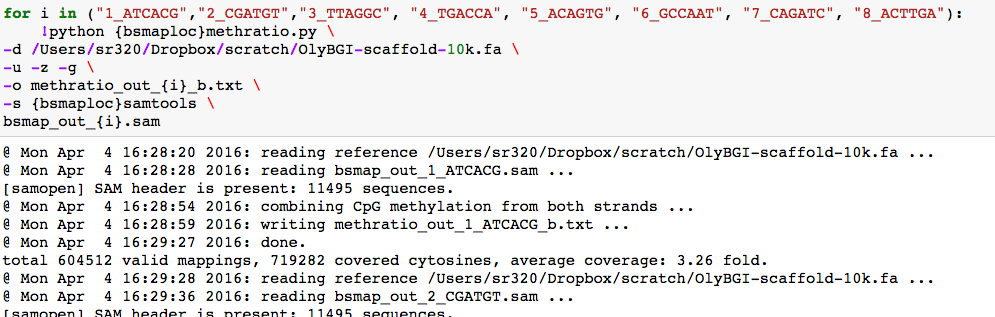
again, making sure there is 10x coverage at a given CG loci
we get

Much weaker if we allow only 3x coverage at a given CG loci

and the bit of R code
setwd("/Volumes/web-1/halfshell/working-directory/16-04-05")
library(methylKit)
file.list ‘mkfmt_2_CGATGT.txt’,
‘mkfmt_3_TTAGGC.txt’,
‘mkfmt_4_TGACCA.txt’,
‘mkfmt_5_ACAGTG.txt’,
‘mkfmt_6_GCCAAT.txt’,
‘mkfmt_7_CAGATC.txt’,
‘mkfmt_8_ACTTGA.txt’
)
myobj=read(file.list,sample.id=list(“1″,”2″,”3″,”4″,”5″,”6″,”7″,”8″),assembly=”Pat10k”,treatment=c(0,0,0,0,1,1,1,1))
meth<-unite(myobj)
head(meth)
nrow(meth)
getCorrelation(meth,plot=F)
hc PCA<-PCASamples(meth)
Recent Comments