Posted by & filed under Cgigas DNA Methylation.

Finally re-getting around to examing our MBD-array data in the context of RNA-seq data. Briefly we have three oysters that were heat shocked with samples taken prior to, and following. An MBD-array experiment was carried out where for each oyster we have information on 50bp genome features (selected probes on the array) whether the region was hypomethylated, hypermethylated or did not change.

Following heat shock approximately 10k differentially methylated features (value >/= 1.8) were identified in all oysters. For all oysters a majority of the features were hypomethylated. Specifically, for oysters #2, #4, and #6 the number of hypomethylated features was 7224, 6560, and 7645, respectively. When only features were considered where at least 3 adjacent probes were also differentially methylated the number of features (merged) for oysters #2, #4, and #6 was 112, 58, and 62, respectively. A majority of these features were hypomethylated (108, 48, and 53, respectively)

Oyster Hypo-methylated Hyper-methylated Hypo-3plus-merged Hypo-3plus-merged
2 7224 2803 108 4
4 6560 3587 48 10
6 7645 4044 53 9

The files with differentially methylated region (DMRs) as defined by value >/= 1.8 are name as 2014.07.02.6M_sig.bedGraph and have the following format (ie head output)

track type=bedGraph name="6M_sig" description="6M_sig" visibility=full color=100,100,0 altColor=0,100,200 priority=20
scaffold1   54599   54654   -1.38187662416007
scaffold1   162129  162191  1.85685479189849
scaffold1   163536  163586  -1.15032035523765
scaffold1   172654  172714  1.33561271440876
scaffold1   174287  174343  -1.62903936976887
scaffold1   178075  178128  1.42323539316231
scaffold1   178685  178740  1.30886296151914
scaffold1   184271  184330  -1.20699853451878
scaffold1   184661  184715  -1.61107459826899

As part of the data provided by the core facility we also obtained genome feature files where there were three or more adjacent signficant probes. The naming structure is 2014.07.02.4M_Hypo_3plusAdjactentProbes.gff with the file format:

scaffold100 804406  804960
scaffold1018    367127  367319
scaffold1018    367618  367674
scaffold1077    401205  401534
scaffold12  244080  244376
scaffold1324    356489  356781

To merge these adjacent features I ran bedtools merge. For example

bedtools merge -d 100 -i 
./data/2014.07.02.colson/genomeBrowserTracks/threeOrMoreAdjacentSigProbes/2014.07.02.2M_Hypo_3plusAdjactentProbes.gff 
> ./analyses/2M_3plusmerge_Hypo.gff 
wc -l ./analyses/2M_3plusmerge_Hypo.gff 

These values are refered to in the above table as Hypo(Hyper)-3plus-merged and the file format:

 scaffold1737   485256  485565
scaffold1894    222981  223032
scaffold1894    223601  223653
scaffold1894    224777  224838
scaffold392 326519  326818
scaffold433 204898  205194
scaffold544 44676   44853
scaffold544 45028   45086
scaffold854 353009  353316

filenames: 6M_3plusmerge_Hypo.bed

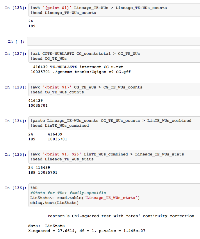
This screenshot shows the different file types
IGV_1A97B149.png

It is important to note that the plusAdjactentProbes.gff files were identified scrictly based on adjacent prove regardless of distance, where the merged files are spatially constrained.

For now I will treat the 6 bed files shown above as the canonical DMRs, for analysis purposes, but I imagine this will change. Hopefully if my IPython notebooks are set up right, this should not be a problem.

These 9 files are available here

2014.07.02.2M_sig.bedGraph  4M_3plusmerge_Hyper.bed
2014.07.02.4M_sig.bedGraph  4M_3plusmerge_Hypo.bed
2014.07.02.6M_sig.bedGraph  6M_3plusmerge_Hyper.bed
2M_3plusmerge_Hyper.bed     6M_3plusmerge_Hypo.bed
2M_3plusmerge_Hypo.bed

IPython notebooks used to get here are here.

Posted by & filed under Cgigas DNA Methylation.

In our original effort (bioRxiv doi: http://dx.doi.org/10.1101/012831) we characterized DMLs in relationship to genomic regions, including putative transposable elements. In this case TEs were defined as tandem repeats and targets that had sequence similarity to protein sequences in other species.

Transposable elements were identified using RepeatMasker, a program that screens and annotates interspersed repeats (Smit et al., 1996-2010). Specifically, RepeatProteinMask, was used with repbase which contained 7,445 peptide sequences. RepeatProteinMask also uses Tandem Repeat Finder (Benson, 1999) to identify tandem repeats which were included in the genome feature track. A total of 119,786 features are in the transposable element genome feature file used for analysis in this paper including 61,319 tandem repeat regions and 58,467 transposable elements identified based on sequence similarity.

Analysis was rerun with targets from RepeatProteinMask (via WUBLASTX) and tandem repeats examined separately. Based on this TEs defined as those identified via RepeatProteinMask were more like to possess lineage specific DMLs.

nbviewer_ipython_org_gist_sr320_7196b3d440d40c6fcb9a_Genomic-location-of-DMLs_1A8031EF.png nbviewer_ipython_org_gist_sr320_7196b3d440d40c6fcb9a_Genomic-location-of-DMLs_1A80321A.png


The GitHub repo documenting this effort has been changed to redefine the TE track as those regions identified from RepeatProteinMask. This makes more sense as it is difficult to determine whether a repeat is associated with an actual transposable element.


Posted by & filed under Workflows.

In an effort to streamline CpG O/E determination across various transcriptomes, here is my latest attempt.

tldr; Ahyacinthus =
Developing_CpG_O_E_Workflow___half-shell_1A7E8AA8.png

This is dependent on have GO slim annotations for all genes – for this particular case the annotation pipeline can be seen here.


Posted by & filed under Workflows.

Goal: Use RNA-seq to compare expression between oysters (n=3) pre and post heat shock.


Based on IPlant Collaborative Tutorial

RNA-Seq_tutorial_-_Education__Outreach__and_Training_-_iPlant_Collaborative_Wiki
https://pods.iplantcollaborative.org/wiki/display/eot/RNA-Seq_tutorial


Task 1: Align read data to Crassostrea gigas genome.

Tophat is a specialized alignment software for RNA-seq reads that is aware of splice junctions when aligning to a reference assembly.

1) Click Apps from DE workspace and select TopHat2-SE. Use search bar.

_18__Discovery_Environment_1A446EF5.png

2) Under ‘Analysis Name’ leave as defaults for make any changes.

3) Under Input data for FASTQ files add six fastq.gz files localed in austral-data with prefixes 2M, 2M-HS, 4M, 4M-HS, 6M, 6M-HS.

4) Under Reference Genome for ‘Provide a reference genome file in FASTA format’ select /austral-data/Crassostrea_gigas.GCA_000297895.1.24.dna_sm.toplevel.fa

5) For Reference Annoations add the GTF file /austral-data/Crassostrea_gigas.GCA_000297895.1.24.gtf

6) Click Launch Analyses and monitor the status of you job.

7) Once complete….

  • Note this takes ~10 hours

Task 2: Assemble transcripts using Cufflinks2

Cufflinks assembles RNA-Seq alignments into a parsimonious set of transcripts, then estimates the relative abundances of these transcripts based on how many reads support each one, taking into account biases in library preparation protocols. A detailed manual can be found at http://cufflinks.cbcb.umd.edu/manual.html.

1) Open Cufflinks2

2) For Input Data add the six bam files from the bam subdirectory of the TopHat2 output.

3) Under Reference Sequence use custom option select /austral-data/Crassostrea_gigas.GCA_000297895.1.24.dna_sm.toplevel.fa

4) For Reference Annoations add the GTF file /austral-data/Crassostrea_gigas.GCA_000297895.1.24.gtf

5) Click Launch Analyses and monitor the status of you job.

  • Note this takes ~2 hours

Task 3: Merge all Cufflinks transcripts into a single transcriptome annotation file using Cuffmerge2

Cuffmerge merges together several Cufflinks assemblies. It handles also handles running Cuffcompare. The main purpose of this application is to make it easier to make an assembly GTF file suitable for use with Cuffdiff. A merged, empirical annotation file will be more accurate than using the standard reference annotation, as the expression of rare or novel genes and alternative splicing isoforms seen in this experiment will be better reflected in the empirical transcriptome assemblies.

1) Open the Cuffmerge2 app. Under ‘Input Data’, browse to the results of the cufflinks analyses (abovee) and add the 6 gtf files located in the gtf subdirectory.

2) For Reference Annoations add the GTF file /austral-data/Crassostrea_gigas.GCA_000297895.1.24.gtf

3) Under Reference Sequence use custom option select /austral-data/Crassostrea_gigas.GCA_000297895.1.24.dna_sm.toplevel.fa

4) Click Launch Analyses and monitor the status of you job.

Task 4: Compare expression analysis using CuffDiff2

Cuffdiff is a program that uses the Cufflinks transcript quantification engine to calculate gene and transcript expression levels in more than one condition and test them for significant differences. http://cufflinks.cbcb.umd.edu/manual.html

1) Open Cuffdiff2. For ‘Input Data’ Sample 1 Name enter Pre adn add three bam file from Tophat analysis..

_39__Discovery_Environment_1A462B43.png

For Sample 2 enter post and add other three bam files …

_39__Discovery_Environment_1A462B91.png

2) Next, open the Reference Annotations section and add a custom reference annotation file using the merged_with_ref_ids.gtf file from the cuffmerge output folder.

3) Click Launch Analyses and monitor the status of you job.