Identifying Differentially Expressed Trinity Transcripts

Using edgeR without replicates:

Be sure to have a samples_described.txt file that describes the relationship between samples and replicates. For example:

where condA-rep1, condA-rep2, condB-rep1, etc…, are all column names in the counts.matrix generated earlier (see top of page). Your sample names that group the replicates are user-defined here.

Using edgeR with replicates:

The above differential expression studies are based on statistics that leverage the raw counts. For studies beyond identifying statistically significant differences in gene expression for individual genes or transcripts between samples, we need to compute the expression values for these features. The number of reads observed for a given feature depends on several factors including the depth of sequencing, the length of the feature (longer transcripts generate more fragment reads), and the expression level of the feature. Expression values normalized for each of these factors are measured in FPKM (fragments per feature kilobase per million reads mapped). The term feature is used here because it could be a transcript, a gene, an exon, or just about anything that can be quantified as a mappable unit. Also, before computing FPKM values, we must normalize the RNA-Seq count data to make them comparable across the muliple samples and replicates. We first use TMM normalization to account for differences in the mass composition of the RNA-seq samples, which doesn’t change the fragment count data, but instead provides a scaling parameter that yields an effective library size (total mappable reads) for each sample. This effective library size is then used in the FPKM calculations.

Compute the TMM-normalized FPKM values for all samples like so:

First, extract the transcript length information from one of the RSEM output files like so:

Using the counts.matrix file created above, perform TMM normalization and generate the FPKM values per transcript and sample as follows:

The above should generate a file: counts.matrix.TMM_normalized.FPKM (adding a suffix to your --matrix filename), which can be used for downstream analyses such as for clustering transcripts based on expression profiles and generating heatmaps (see below).

An initial step in analyzing differential expression is to extract those transcripts that are most differentially expressed (most significant P-values and fold-changes) and to cluster the transcripts according to their patterns of differential expression across the samples. To do this, you can run the following from within the edgeR output directory, bu running the following script:

For example:

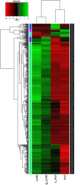
The above is mostly just a visual reference. To more seriously study and define your gene clusters, you will need to interact with the data as described below. The clusters and all required data for interrogating and defining clusters is all saved with an R-session, locally with the file all.RData. This will be leveraged as described below.

Run the script below to automatically split the data set into a sets of transcripts with related expression patterns by partitioning the hierarchically clustered transcript tree.

For example:

A directory will be created called: diffExpr.P0.001_C2.matrix.R.all.RData.clusters_fixed_P_20/ and contain the expression matrix for each of the clusters (log2-transformed, median centered).

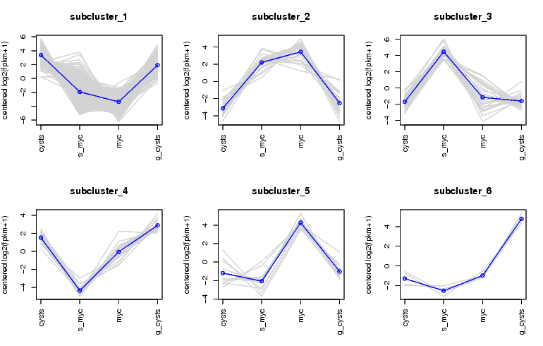
To plot the mean-centered expression patterns for each cluster, visit that directory and run:

This will generate a summary image file: my_cluster_plots.pdf, as shown below:

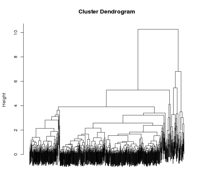
Manually defining your clusters is the best way to organize the data to your liking. This is an interactive process. Fire up R from within your output directory, being sure it contains the all.RData file, and enter the following commands:

This should yield a display containing the hierarchically clustered genes, as shown below:

Now, manually define your clusters from left to right (order matters here, so you can decipher the results later!) by clicking on the branch vertical branch that defines the clade of interest. After clicking on the branch, it will be drawn with a red box around the selected clade, as shown below:

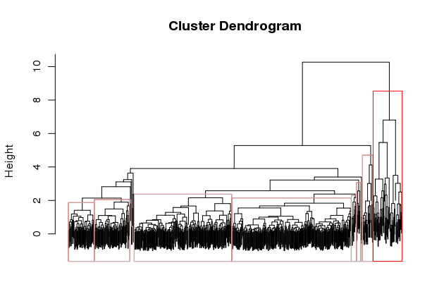
Right click with the mouse (or double-touch a touchpad) to exit from cluster selection.

The clusters as selected will be written to a subdirectory manually_defined_clusters_$count_clusters, and exist in a format similar to the automated-selection of clusters described above. Likewise, you can generate plots of the expression patterns for each cluster using the plot_expression_patterns.pl script.