Tag Archives: bismark

DNA Methylation Analysis – Olympia Oyster Whole Genome BSseq Bismark Pipeline Comparison

Ran Bismark using our high performance computing (HPC) node, Mox, with two different bowtie2 settings:

  1. Default settings

  2. –score_min L,0,-0.6

The second setting is a bit less stringent than the default settings and should result in a higher percentage of reads mapping. However, not entirely sure what the actual implications will be (if any) for interpreting the resulting data.

Input data was previously trimmed per Bismark’s recommendation for Illumina TruSeq libraries (TrimGalore! 5′ 10bp):

List of input files and Bismark configurations can be seen in the SLURM scripts:


RESULTS

Output folders:

DNA Methylation Analysis – Olympia oyster BSseq MethylKit Analysis

NOTE: IMPORTANT CAVEATS – READ POST BEFORE USING DATA.
I’m posting this for posterity and to provide an overview of what (and whatnot) to do. Plus, this has a good R script for using MethylKit that can be used for subsequent analyses.

The goal of this analysis was to compare the methylation profiles of Olympia oysters originating from a common population (Fidalgo Bay) that were raised in two different locations (Fidalgo Bay & Oyster Bay).

An overview of the experiment can be viewed here:

I previously ran all of Olympia oyster DNA methylation sequencing data through the Bismark pipeline, and then processed them using the MethylKit R library.

First mistake (Bismark):

  • Trimmed FastQ files “incorrectly”.

Bismark provides an excellent user guide and provides a handy table on how to decide on trimming parameters, but I mistakenly trimmed these according to the recommendations for a different library preparation technique. I trimmed based on the Zymo Pico-Methyl Kit (which was used for the other group of data that I processed simultaneously), instead of the TruSeq library prep.

So, “incorrectly” isn’t necessarily the proper term here. The analysis can still be used, however, it’s likely that the excessive trimming results in reducing sequencing coverage, and, in turn, making the downstream analysis result in a highly conservative output. Thus, the data isn’t wrong or bad, it is just very limited.

And, this leads to the second mistake (Bismark):

  • Bowtie alignment score too strict

There’s a bit of a weird “battle” between Bismark and bowtie2. Bismark uses bowtie2 for generating alignments, but bowtie2’s default cutoff score overrides Bismark’s. So, to adjust the score value, you have to explicitly add the scoring parameters to your Bismark parameters during the alignment step. I did not do this.

Again, it’s not wrong, per se, but leads to a significantly limited set of data in the final analysis.

The data were analyzed based on a minimum of:

  • 3x coverage

  • 25% difference in methylation


RESULTS:

Methylkit analysis (R project; GitHub):

BedGraph file (BED):

The analysis resulted in a total of seven (yes, 7) differentially methylated loci (DML) between the two groups. It was this result that made Steven and me revisit the initial Bismark analysis. He has done this previously (but differently) and gotten significantly greater numbers of DML.

Knowing all of this, I will re-trim the data and adjust Bismark alignment score thresholds and then re-analyze with MethylKit.

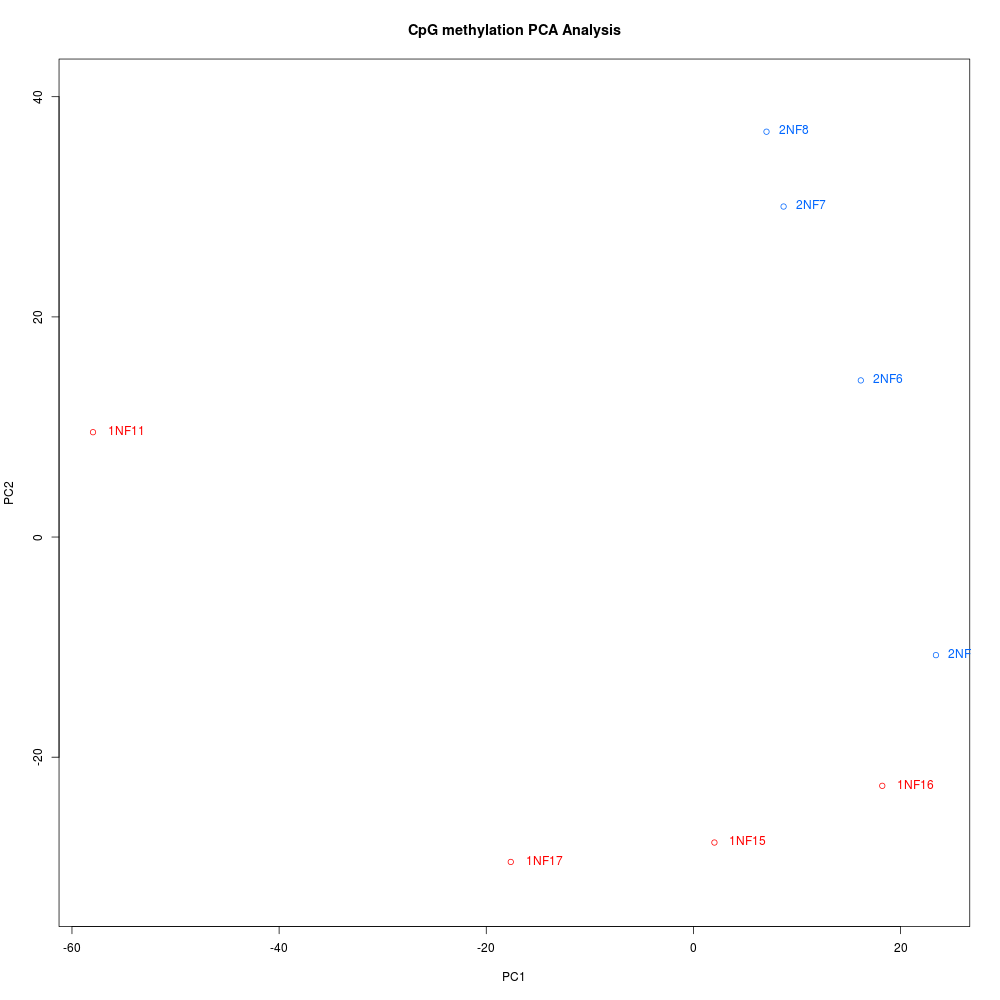
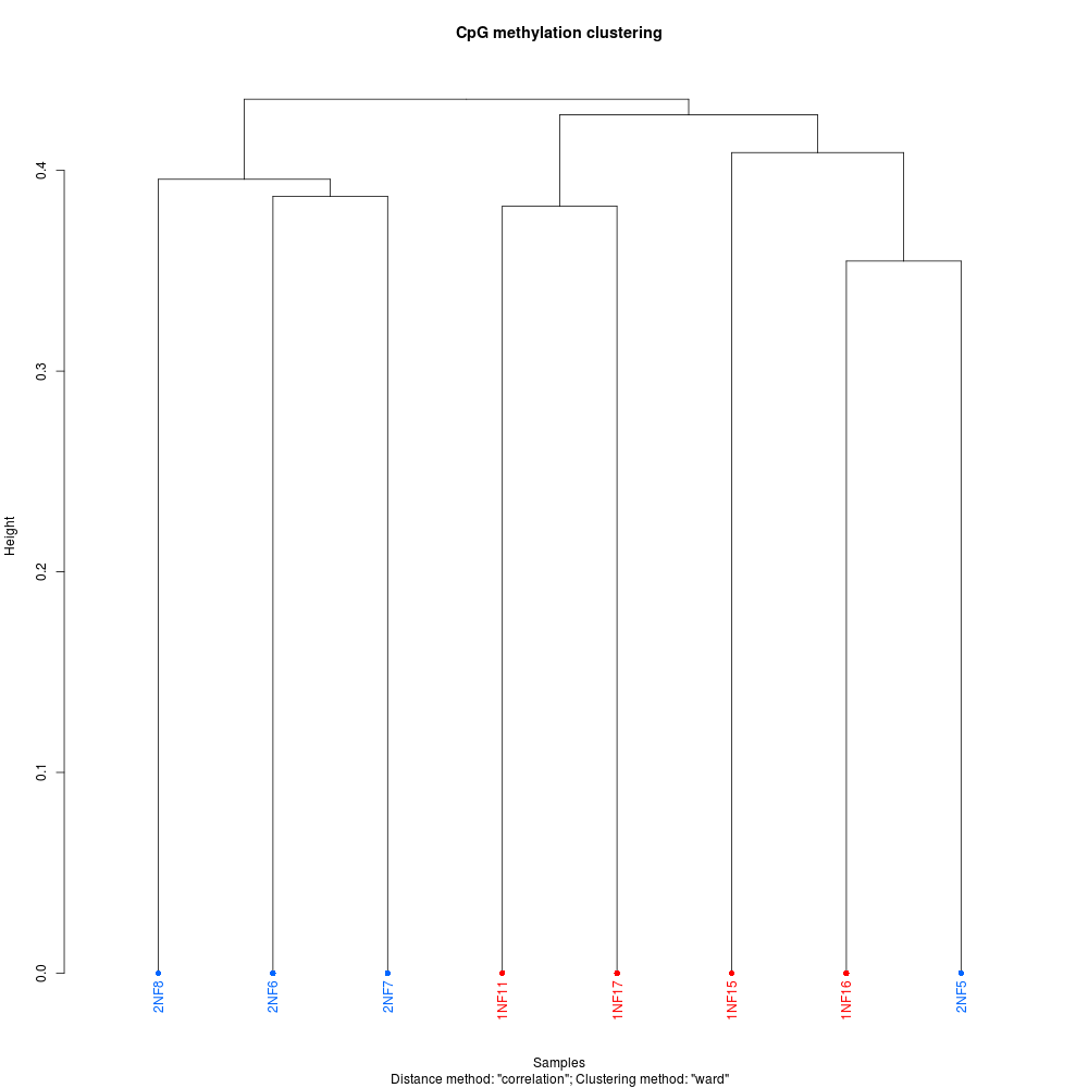
Regardless here’re some plots to add some visual flair to this notebook entry (these, and more, are available in the GitHub repo):

CLUSTERING DENDROGRAM


PCA PLOT

DNA Methylation Analysis – Bismark Pipeline on All Olympia oyster BSseq Datasets

Bismark analysis of all of our current Olympia oyster (Ostrea lurida) DNA methylation high-throughput sequencing data.

Analysis was run on Emu (Ubuntu 16.04LTS, Apple Xserve). The primary analysis took ~14 days to complete.

All operations are documented in a Jupyter notebook (GitHub):

Genome used:


Input files ( see Olympia oyster Genomic GitHub wiki for more info ):

WG BSseq of Fidalgo Bay offspring grown in Fidalgo Bay & Oyster Bay
  • 1_ATCACG_L001_R1_001.fastq.gz

  • 2_CGATGT_L001_R1_001.fastq.gz

  • 3_TTAGGC_L001_R1_001.fastq.gz

  • 4_TGACCA_L001_R1_001.fastq.gz

  • 5_ACAGTG_L001_R1_001.fastq.gz

  • 6_GCCAAT_L001_R1_001.fastq.gz

  • 7_CAGATC_L001_R1_001.fastq.gz

  • 8_ACTTGA_L001_R1_001.fastq.gz

MBDseq of two populations (Hood Canal & Oyster Bay) grown in Clam Bay
  • zr1394_10_s456.fastq.gz

  • zr1394_11_s456.fastq.gz

  • zr1394_12_s456.fastq.gz

  • zr1394_13_s456.fastq.gz

  • zr1394_14_s456.fastq.gz

  • zr1394_15_s456.fastq.gz

  • zr1394_16_s456.fastq.gz

  • zr1394_17_s456.fastq.gz

  • zr1394_18_s456.fastq.gz

  • zr1394_1_s456.fastq.gz

  • zr1394_2_s456.fastq.gz

  • zr1394_3_s456.fastq.gz

  • zr1394_4_s456.fastq.gz

  • zr1394_5_s456.fastq.gz

  • zr1394_6_s456.fastq.gz

  • zr1394_7_s456.fastq.gz

  • zr1394_8_s456.fastq.gz

  • zr1394_9_s456.fastq.gz


RESULTS:

With Bismark complete, these two sets of analyses can now be looked into further (and separately, as they are separate experiments) using things like MethylKit (R package) and
the Integrative Genomics Viewer (IGV).

Output folder:

Bismark Summary Report:

Individual Sample Reports:

TrimGalore/FastQC/MultiQC – TrimGalore! RRBS Geoduck BS-seq FASTQ data


20180516 – UPDATE!!

THIS WAS RUN WITH THE INCORRECT SETTING IN TRIMGALORE! --non-directional

WILL RE-RUN


Steven requested that I trim the Geoduck RRBS libraries that we have, in preparation to run them through Bismark.

These libraries were originally created by Hollie Putnam using the TruSeq DNA Methylation Kit (Illumina):

All analysis is documented in a Jupyter Notebook; see link below.

Overview of process:

  1. Copy EPI* FastQ files from owl/P_generosa to roadrunner.

  2. Confirm data integrity via MD5 checksums.

  3. Run TrimGalore! with --paired, --rrbs, and --non-directional settings.

  4. Run FastQC and MultiQC on trimmed files.

  5. Copy all data to owl (see Results below for link).

  6. Confirm data integrity via MD5 checksums.

Jupyter Notebook:


Results:
TrimGalore! output folder:
FastQC output folder:
MultiQC output folder:
MultiQC report (HTML):

BS-seq Mapping – Olympia oyster bisulfite sequencing: TrimGalore > FastQC > Bismark

Steven asked me to evaluate our methylation sequencing data sets for Olympia oyster.

According to our Olympia oyster genome wiki, we have the following two sets of BS-seq data:

All computing was conducted on our Apple Xserve: emu.

All steps were documented in this Jupyter Notebook (GitHub): 20180503_emu_oly_methylation_mapping.ipynb

NOTE: The Jupyter Notebook linked above is very large in size. As such it will not render on GitHub. It will need to be downloaded to a computer that can run Jupyter Notebooks and viewed that way.

Here’s a brief overview of what was done.

Samples were trimmed with TrimGalore and then evaluated with FastQC. MultiQC was used to generate a nice visual summary report of all samples.

The Olympia oyster genome assembly, pbjelly_sjw_01, was used as the reference genome and was prepared for use in Bismark:


/home/shared/Bismark-0.19.1/bismark_genome_preparation \
--path_to_bowtie /home/shared/bowtie2-2.3.4.1-linux-x86_64/ \
--verbose /home/sam/data/oly_methylseq/oly_genome/ \
2> 20180507_bismark_genome_prep.err

Bismark was run on trimmed samples with the following command:


/home/shared/Bismark-0.19.1/bismark \
--path_to_bowtie /home/shared/bowtie2-2.3.4.1-linux-x86_64/ \
--genome /home/sam/data/oly_methylseq/oly_genome/ \
-u 1000000 \
-p 16 \
--non_directional \
/home/sam/analyses/20180503_oly_methylseq_trimgalore/1_ATCACG_L001_R1_001_trimmed.fq.gz \
/home/sam/analyses/20180503_oly_methylseq_trimgalore/2_CGATGT_L001_R1_001_trimmed.fq.gz \
/home/sam/analyses/20180503_oly_methylseq_trimgalore/3_TTAGGC_L001_R1_001_trimmed.fq.gz \
/home/sam/analyses/20180503_oly_methylseq_trimgalore/4_TGACCA_L001_R1_001_trimmed.fq.gz \
/home/sam/analyses/20180503_oly_methylseq_trimgalore/5_ACAGTG_L001_R1_001_trimmed.fq.gz \
/home/sam/analyses/20180503_oly_methylseq_trimgalore/6_GCCAAT_L001_R1_001_trimmed.fq.gz \
/home/sam/analyses/20180503_oly_methylseq_trimgalore/7_CAGATC_L001_R1_001_trimmed.fq.gz \
/home/sam/analyses/20180503_oly_methylseq_trimgalore/8_ACTTGA_L001_R1_001_trimmed.fq.gz \
/home/sam/analyses/20180503_oly_methylseq_trimgalore/zr1394_10_s456_trimmed.fq.gz \
/home/sam/analyses/20180503_oly_methylseq_trimgalore/zr1394_11_s456_trimmed.fq.gz \
/home/sam/analyses/20180503_oly_methylseq_trimgalore/zr1394_12_s456_trimmed.fq.gz \
/home/sam/analyses/20180503_oly_methylseq_trimgalore/zr1394_13_s456_trimmed.fq.gz \
/home/sam/analyses/20180503_oly_methylseq_trimgalore/zr1394_14_s456_trimmed.fq.gz \
/home/sam/analyses/20180503_oly_methylseq_trimgalore/zr1394_15_s456_trimmed.fq.gz \
/home/sam/analyses/20180503_oly_methylseq_trimgalore/zr1394_16_s456_trimmed.fq.gz \
/home/sam/analyses/20180503_oly_methylseq_trimgalore/zr1394_17_s456_trimmed.fq.gz \
/home/sam/analyses/20180503_oly_methylseq_trimgalore/zr1394_18_s456_trimmed.fq.gz \
/home/sam/analyses/20180503_oly_methylseq_trimgalore/zr1394_1_s456_trimmed.fq.gz \
/home/sam/analyses/20180503_oly_methylseq_trimgalore/zr1394_2_s456_trimmed.fq.gz \
/home/sam/analyses/20180503_oly_methylseq_trimgalore/zr1394_3_s456_trimmed.fq.gz \
/home/sam/analyses/20180503_oly_methylseq_trimgalore/zr1394_4_s456_trimmed.fq.gz \
/home/sam/analyses/20180503_oly_methylseq_trimgalore/zr1394_5_s456_trimmed.fq.gz \
/home/sam/analyses/20180503_oly_methylseq_trimgalore/zr1394_6_s456_trimmed.fq.gz \
/home/sam/analyses/20180503_oly_methylseq_trimgalore/zr1394_7_s456_trimmed.fq.gz \
/home/sam/analyses/20180503_oly_methylseq_trimgalore/zr1394_8_s456_trimmed.fq.gz \
/home/sam/analyses/20180503_oly_methylseq_trimgalore/zr1394_9_s456_trimmed.fq.gz \
2> 20180507_bismark_02.err

Results:

TrimGalore output folder:

FastQC output folder:

MultiQC output folder:

MultiQC Report (HTML):

Bismark genome folder: 20180503_oly_genome_pbjelly_sjw_01_bismark/

Bismark output folder:


Whole genome BS-seq (2015)

Prep overview
  • Library prep: Roberts Lab
  • Sequencing: Genewiz
Bismark Report Mapping Percentage
1_ATCACG_L001_R1_001_trimmed_bismark_bt2_SE_report.txt 40.3%
2_CGATGT_L001_R1_001_trimmed_bismark_bt2_SE_report.txt 39.9%
3_TTAGGC_L001_R1_001_trimmed_bismark_bt2_SE_report.txt 40.2%
4_TGACCA_L001_R1_001_trimmed_bismark_bt2_SE_report.txt 40.4%
5_ACAGTG_L001_R1_001_trimmed_bismark_bt2_SE_report.txt 39.9%
6_GCCAAT_L001_R1_001_trimmed_bismark_bt2_SE_report.txt 39.6%
7_CAGATC_L001_R1_001_trimmed_bismark_bt2_SE_report.txt 39.9%
8_ACTTGA_L001_R1_001_trimmed_bismark_bt2_SE_report.txt 39.7%

MBD BS-seq (2015)

Prep overview
  • MBD: Roberts Lab
  • Library prep: ZymoResearch
  • Sequencing: ZymoResearch
Bismark Report Mapping Percentage
zr1394_1_s456_trimmed_bismark_bt2_SE_report.txt 33.0%
zr1394_2_s456_trimmed_bismark_bt2_SE_report.txt 34.1%
zr1394_3_s456_trimmed_bismark_bt2_SE_report.txt 32.5%
zr1394_4_s456_trimmed_bismark_bt2_SE_report.txt 32.8%
zr1394_5_s456_trimmed_bismark_bt2_SE_report.txt 35.2%
zr1394_6_s456_trimmed_bismark_bt2_SE_report.txt 35.5%
zr1394_7_s456_trimmed_bismark_bt2_SE_report.txt 32.8%
zr1394_8_s456_trimmed_bismark_bt2_SE_report.txt 33.0%
zr1394_9_s456_trimmed_bismark_bt2_SE_report.txt 34.7%
zr1394_10_s456_trimmed_bismark_bt2_SE_report.txt 34.9%
zr1394_11_s456_trimmed_bismark_bt2_SE_report.txt 30.5%
zr1394_12_s456_trimmed_bismark_bt2_SE_report.txt 35.8%
zr1394_13_s456_trimmed_bismark_bt2_SE_report.txt 32.5%
zr1394_14_s456_trimmed_bismark_bt2_SE_report.txt 30.8%
zr1394_15_s456_trimmed_bismark_bt2_SE_report.txt 31.3%
zr1394_16_s456_trimmed_bismark_bt2_SE_report.txt 30.7%
zr1394_17_s456_trimmed_bismark_bt2_SE_report.txt 32.4%
zr1394_18_s456_trimmed_bismark_bt2_SE_report.txt 34.9%