Tag Archives: docker

Assembly Comparisons – Olympia oyster genome assemblies

— UPDATE 20171009 —

Having run through this a bunch of times now, I realized that the analysis below incorrectly identifies the outputs from Sean’s Redundans runs. The correct output from each of those runs should be the “scaffolds.reduced.fa” FAST files. The “contigs.fa” files that I linked to below are actually the assemblies produced by other programs; which are required as an input for Redudans.


I recently completed an assembly of the UW PacBio sequencing data using Racon and wanted some assembly stats, as well as a way to compare this assembly to the assemblies Sean had completed.

Additionally, Steven recently performed an assembly comparison and I noticed he got some odd results. Specifically, of the three assemblies he compared (PacBio x 1, Illumina x 2), both of the Illumina assemblies had a large quantity of “Ns” in the assemblies. This didn’t seem right and the comparison program he used (QUAST) spit out a message indicating that it seemed like scaffolds were used, instead of contigs. So, I thought I’d give it a shot and see if I could track down non-scaffolded assemblies produced by Sean.

Jupyter notebook (GitHub): 20171003_docker_oly_assembly_comparisons.ipynb

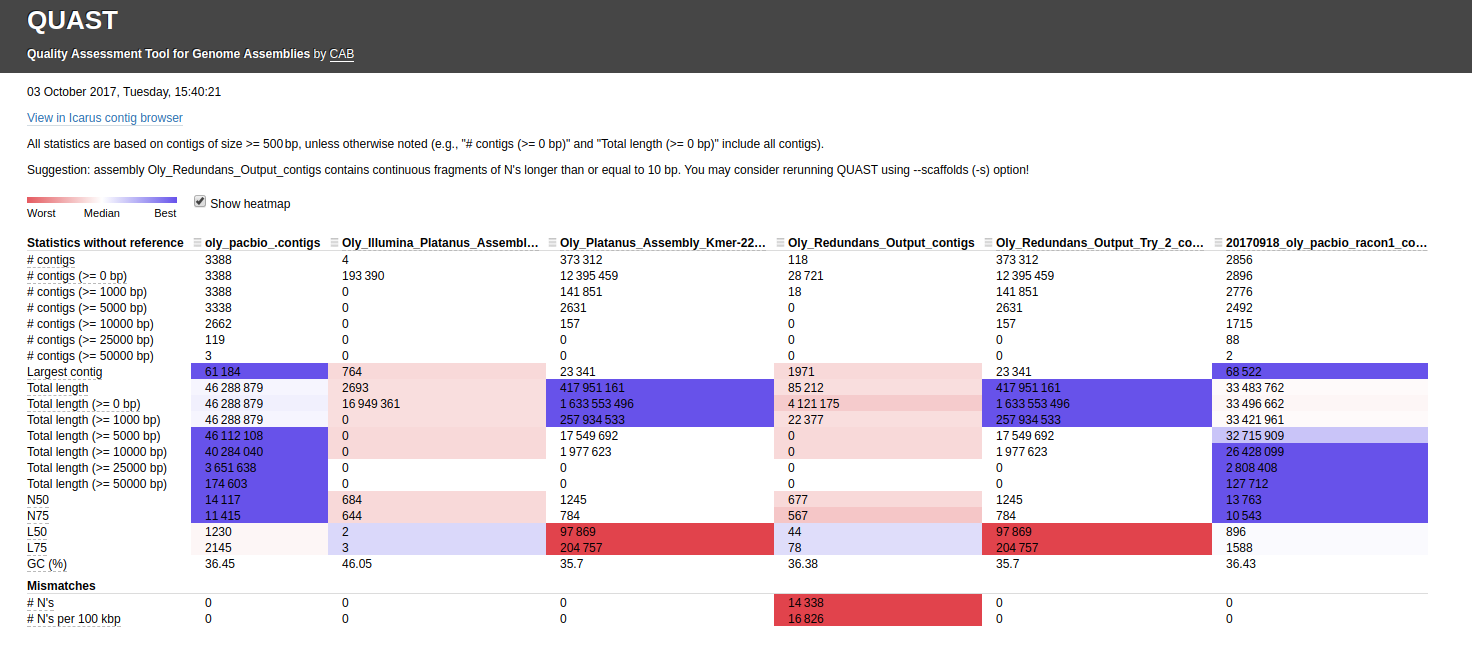
First, I compared the following six assemblies (FASTA files) using QUAST:

Sean’s Assemblies:

Sam’s Assembly:

QUAST output directory: http://owl.fish.washington.edu/Athaliana/20171003_quast_oly_genome_assemblies/

Here’s the assembly comparison of all assemblies (click on image for larger view):

Interactive version of that graphic is here: http://owl.fish.washington.edu/Athaliana/20171003_quast_oly_genome_assemblies/report.html

The first thing that jumps out to me is the fact that two of the Illumina assemblies, which used different assemblers(!!) have the EXACT same assembly stats. This occurrence seems extremely unlikely. I’ve double-checked my Jupyter notebook to make sure that I didn’t assign the same file by accident (see Input #6)

Very strange!

I also noticed that the first Redundans assembly of Sean’s has a ton of “Ns”, suggesting that it’s actually a scaffolded assembly. As with Steven’s QUAST run, QUAST spits out the messages suggesting to use the “–scaffold” option for this file.

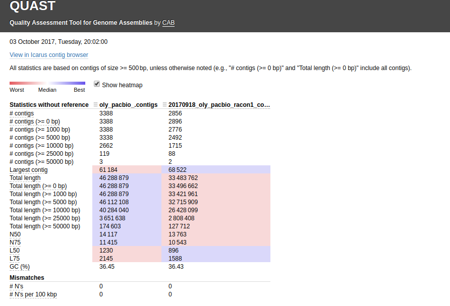
The other thing I noticed is the two PacBio assemblies (Canu & Racon) have a huge difference in the total number of bp (~13,000,000)! I ran a QUAST assembly comparison between just those two for easier viewing/comparison (http://owl.fish.washington.edu/Athaliana/20171003_quast_oly_pacbio_assemblies/):

Interactive version of that graphic is here: http://owl.fish.washington.edu/Athaliana/20171003_quast_oly_pacbio_assemblies/report.html

The fact that there is such a large discrepancy in the total number of bps between these two assemblies really leaves me to believe that I am missing a FASTQ file from my assembly. I’m going to go back and see if that is indeed the case or if this difference in the assemblies is real.

Here’s an embedded version of my Jupyter notebook:

FASTQC – Oly BGI GBS Raw Illumina Data Demultiplexed

Last week, I ran the two raw FASTQ files through FastQC. As expected, FastQC detected “errors”. These errors are due to the presence of adapter sequences, barcodes, and the use of a restriction enzyme (ApeKI) in library preparation. In summary, it’s not surprising that FastQC was not please with the data because it’s expecting a “standard” library prep that’s already been trimmed and demultiplexed.

However, just for comparison, I ran the demultiplexed files through FastQC. The Jupyter notebook is linked (GitHub) and embedded below. I recommend viewing the Jupyter notebook on GitHub for easier viewing.

Results:

Pretty much the same, but with slight improvements due to removal of adapter and barcode sequences. The restriction site still leads to FastQC to report errors, which is expected.

Links to all of the FastQC output files are linked at the bottom of the notebook.

Jupyter notebook (GitHub): 20170306_docker_fastqc_demultiplexed_bgi_oly_gbs.ipynb

Data Received – Jay’s Coral RADseq and Hollie’s Geoduck Epi-RADseq

Jay received notice from UC Berkeley that the sequencing data from his coral RADseq was ready. In addition, the sequencing contains some epiRADseq data from samples provided by Hollie Putnam. See his notebook for multiple links that describe library preparation (indexing and barcodes), sample pooling, and species breakdown.

For quickest reference, here’s Jay’s spreadsheet with virtually all the sample/index/barcode/pooling info (Google Sheet): ddRAD/EpiRAD_Jan_16

I’ve downloaded both the demultiplexed and non-demultiplexed data, verified data integrity by generating and comparing MD5 checksums, copied the files to each of the three species folders on owl/nightingales that were sequenced (Panopea generosa, Anthopleura elegantissima, Porites astreoides), generated and compared MD5 checksums for the files in their directories on owl/nightingales, and created/updated the readme files in each respective folder.


Data management is detailed in the Jupyter notebook below. The notebook is embedded in this post, but it may be easier to view on GitHub (linked below).

Readme files were updated outside of the notebook.

Jupyter notebook (GitHub): 20170227_docker_jay_ngs_data_retrieval.ipynb

Data Analysis – Initial O.lurida Fst Determination from GBS Data

Finally running some analysis on the output from my PyRad analysison 20160727.

I’m following Katherine Silliman’s Jupyter notebook (2bRAD Subset Population Structure Analysis.ipynb) as a guide.

The initial analysis (which isn’t much) is in the Jupyter notebook below. The analysis will be continued on a later date.

Jupyter notebook: 20161117_docker_oly_vcf_analysis.ipynb

I’ve embedded the notebook below, but it’s much easier to view (there are many lengthy commands/filenames that wrap lines in the embedded version below) the actual file linked above.

Data Management – Tracking O.lurida FASTQ File Corruption

UPDATE 20170104 – These two corrupt files have been replaced with non-corrupt files.


Sean identified an issue with one of the original FASTQ files provided to use by BGI. Additionally, Steven had (unknowingly) identified the same corrupt file, as well as a second corrupt file in the set of FASTQ files. The issue is discussed here: https://github.com/sr320/LabDocs/issues/334

Steven noticed the two files when he ran the program FASTQC and two files generated no output (but no error message!).

The two files in question are:

  • 151118_I137_FCH3KNJBBXX_L5_wHAXPI023905-96_1.fq.gz
  • 151114_I191_FCH3Y35BCXX_L2_wHAMPI023991-66_2.fq.gz

This post is an attempt to document where things went wrong, but having glanced through this data a bit already, it won’t provide any answers.

I originally downloaded the data on 20160127 to my home folder on Owl (this is detailed in the Jupyter notebook in that post) and generated/compared MD5 checksum values. The values matched at that time.

So, let’s investigate a bit further…

Launch Docker container

docker run - p 8888:8888 -v /Users/sam/data/:/data -v /Users/sam/owl_home/:/owl_home -v /Users/sam/owl_web/:owl_web -v /Users/sam/gitrepos/LabDocs/jupyter_nbs/sam/:/jupyter_nbs -it 0ba43904567e

The command allows access to Jupyter Notebook over port 8888 and makes my Jupyter Notebook GitHub repo and my data files accessible to the Docker container.

Once the container was started, started Jupyter Notebook with the following command inside the Docker container:

jupyter notebook

This command is configured in the Docker container to launch a Jupyter Notebook without a browser on port 8888.

Jupyter notebook file: 20161117_docker_oly_genome_fastq_corruption.ipynb

I’ve embedded the notebook below, but it’s much easier to view (there are many lengthy commands/filenames that wrap lines in the embedded version below) the actual file linked above.

Data Analysis – PyRad Analysis of Olympia Oyster GBS Data

Previously, I ran a PyRad analysis on just a subset of these samples in an attempt to have some data for a grant pre-proposal.

I’ve now completed a PyRad analysis on the full set. Now, I just need to figure out what to do with the output from this…

Jupyter Notebook: 20160715_ec2_oly_gbs_pyrad.ipynb

Docker – VirtualBox Defaults on OS X

I noticed a discrepancy between what system info is detected natively on Roadrunner (Apple Xserve) and what was being shown when I started a Docker container.

Here’s what Roadrunner’s system info looks like outside of a Docker container:


However, here’s what is seen when running a Docker container:


It’s important to notice the that the Docker container is only seeing 2 CPUs. Ideally, the Docker container would see that this system has 8 cores available. By default, however, it does not. In order to remedy this, the user has to adjust settings in VirtualBox. VirtualBox is a virtual machine thingy that gets installed with the Docker Toolbox for OS X. Apparently, Docker runs within VirtualBox, but this is not really transparent to a beginner Docker user on OS X.

To change the way VirtualBox (and, in turn, Docker) can access the full system hardware, you must launch the VirtualBox application (if you installed Docker using Docker Toolbox, you should be able to find this in your Applications folder). Once you’ve launched VirtualBox, you’ll have to turn off the virtual machine that’s currently running. Once that’s been accomplished, you can make changes and then restart the virtual machine.


Shutdown VirtualBox machine before you can make changes:


Here are the default CPU settings that VirtualBox is using:


Maxed out the CPU slider:


Here are the default RAM settings that VirtualBox is using:


Changed RAM slider to 24GB:


Now, let’s see what the Docker container reports for system info after making these changes:


Looking at the CPUs now, we see it has 8 listed (as opposed to only 2 initially). I think this means that Docker now has full access to the hardware on this machine.

This situation is a weird shortcoming of Docker (and/or VirtualBox). Additionally, I think this issue might only exist on the OS X and Windows versions of Docker, since they require the installation of the Docker Toolbox (which installs VirtualBox). I don’t think Linux installations suffer from this issue.

Docker – One liner to create Docker container

One liner to create Docker container for Jupyter notebook usage and data analysis on roadrunner (Xserve):

docker run -p 8888:8888 -v /Users/sam/gitrepos/LabDocs/jupyter_nbs/sam/:/notebooks -v /Users/sam/data/:/data -v /Users/sam/analysis/:/analysis -it kubu4/bioinformatics:v11 /bin/bash

This does the following:

  • Maps roadrunner port 8888 to Docker container port 8888 (for Jupyter notebook access outside of the Docker container)
  • Mounts my local Jupyter notebooks directory to the
    /notebooks

    directory in the Docker container

  • Mounts my local data directory to the
    /data

    directory in the Docker container

  • Mounts my local analysis directory to the
    /analysis

    directory in the Docker container

These commands allow me to interact with data outside of the Docker container.

Docker – Improving Roberts Lab Reproducibility

In an attempt at furthering our lab’s abilities to maximize our reproducibility, I’ve been  working on developing an all-encompassing Docker image. Docker is a type of virtual machine (i.e. a self-contained computer that runs within your computer). For the Roberts Lab, the advantage of using Docker is that the Docker images can be customized to run a specific suite of software and these images can then be used by any other person in the lab (assuming they can run Docker on their particular operating system), regardless of operating system. In turn, if everyone is using the same Docker image (i.e. the same virtual machine with all the same software), then we should be able to reproduce data analyses more reliably, due to the fact that there won’t be differences between software versions that people are using. Additionally, using Docker greatly simplifies the setup of new computers with the requisite software.

I’ve put together a Dockerfile (a Dockerfile is a text file/script that Docker uses to retrieve software and build a computer image with those specific instructions) which will automatically build a Docker image (i.e. virtual computer) that contains all of the normal bioinformatics software our lab uses. This has been a side project while I wait for Stacks analysis to complete (or, fail, depending on the day) and it’s finally usable! The image that is built from this Dockerfile will even let the user run R Studio and/or Jupyter Notebooks in their browser (I’m excited about this part)!

Here’s the current list of software that will be installed:

bedtools 2.25.0
bismark 0.15.0
blast 2.3.0+
bowtie2 2.2.8
bsmap 2.90
cufflinks 2.1.1
fastqc 0.11.5
fastx_toolkit 0.0.13
R 3.2.5
RStudio Server0.99
pyrad 3.0.66
samtools 0.1.19
stacks 1.40
tophat 2.1.1
trimmomatic 0.36

In order to set this up, you need to install Docker and download the Dockerfile (Dockerfile.bio) I’ve created.

I’ve written a bit of a user guide (specific to this Dockerfile) here to get people started: docker.md

The user guide explains a bit how all of this works and tries to progress from a “basic” this-is-how-to-get-started-with-Docker to an “advanced” description of how to map ports, mount local volumes in your containers, and how to start/attach previously used containers.

The next major goal I have with this Docker project is to get the R kernel installed for Jupyter Notebooks. Currently, the Jupyter Notebook installation is restricted to the default Python 2 kernel.

Additionally, I’d like to improve the usability of the Docker image by setting up aliases in the image. Meaning, a user who wants to use the bowtie program can just type “bowtie”. Currently, the user has to type “bowtie2_2.2.8″ (although, with this being in the system PATH and tab-completion, it’s not that big of a deal), which is a bit ugly.

For some next level stuff, I’d also like to setup all Roberts Lab computers to automatically launch the Docker image when the user opens a terminal. This would greatly simplify things for new lab members. They wouldn’t have to deal with going through the various Docker commands to start a Docker container. Instead, their terminal would just put them directly into the container and the user would be none-the-wiser. They’d be reproducibly conducting data analysis without even having to think about it.