I’ve been working on getting our T5 Excellence titrator (Mettler Toledo) with Rondolino sample changer (Mettler Toledo) set up and operational.

A significant part of the setup process is utilizing the LabX Software (Mettler Toledo, v.8.0.0). The software is vastly overpowered (i.e. overly complicated) for the nature of our work. As such, it’s been quite the struggle to get the titrator to do what we need it to do.

We’ve received a great deal of help and insight from Dr. Hollie Putnam (Univ. of Rhode Island). She provided us with a LabX Method that was previously used by some of her colleagues. In addition, she provided us with an SOP from those colleagues that helps describe how to physically operate the titrator and a corresponding workflow for data collection. Of course, she’s also helped immensely with understanding the entire process of the chemistry to how to process samples to implementing various quality control checks to ensure we’ll get the most accurate data we can.

After some significant struggles with getting the method to work properly, I contacted Mettler Toledo and the technician helped me modify the method that Hollie passed along to us to run properly.

Basic Functionality Fixes

The updated method resolves the following issues we were having (see annotated screenshot below the lists for more detailed overview of method changes):

• Method only ends titration at specified maximum volume instead of specified potential
• Method exits with Sample State = “Not OK”
• Method fails to calculate acid Consumption at end of titration

I also modified the method to bring it up to spec with the Dickson Guide to Best Practices for Ocean CO₂ Measurements- SOP3b:

• Changed method template to use Endpoint (EP) titration instead of Equivalence Point (EQP) titration
• Implemented initial titration step to pH=3.5 (200mV)
• Added degassing step to match Dickson specs (increase stir speed and duration)
• Improved titration precision by changing titration rate to automatically adjust relative to set endpoint values
• Set correct voltages for pH=3.5 (200mV) & pH=3.0 (228.57mV); no need to adjust prior to running method

I recommend opening the image below in a new tab in order to be able to read all of the annotations.

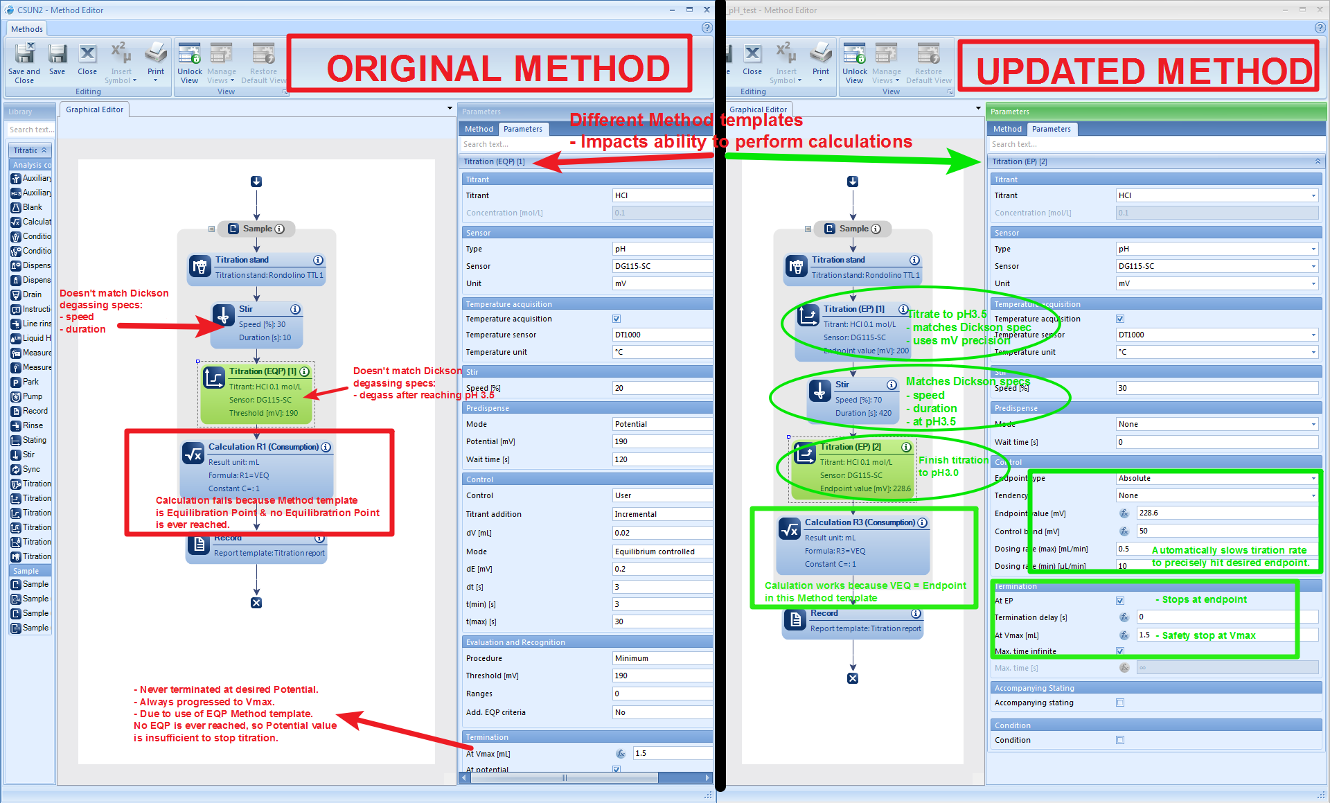
So, all of that stuff makes the method actually run according to the Dickson specs. It also fixes the Consumption calculation. Although this aspect of the method is totally unnecessary (the consumption calculation could easily be integrated in downstream analysis), it feels good to have fixed the issue and learn how that aspect of the LabX software functions.

Data Export Fixes

We recently acquired the necessary license to unlock the ability to export data.

Digression:

This is a terrible practice implemented by Mettler Toledo, btw. I’m particularly annoyed because I specifically asked about data exports when I spoke with the sales rep when initiating the purchase. He neglected to mention that I’d need to purchase an additional license. I wasted a lot of time and hair pulling before I learned that this feature was locked by design and that I needed this additional license.

Anyway, the struggles continued even after activating the license. I was not able to export any data – every attempt at specifying a directory in which to save data failed.

Mettler Toledo informed me that it has to do with Windows Services Permissions.

To change permissions to allow data export:

1. Search Windows for “Services”
2. Open “Services”
3. Right-click on “LabXHostService”
4. Select “Properties”
5. Click “Log On” tab.
6. Click “Local System Account” radio button.
7. Check “Allow service to interact with desktop” box.
8. Restart computer.

Now, the data gets automatically exported to my desired directory as soon as a LabX task is finished!!

Data Management & Informational Resources

As we are very close to beginning to actually collect data with the titrator, I realized that all this data needs to go somewhere. Additionally, people need someplace to find out how to use all of this stuff (equipment, software, etc.).

I created a new GitHub repo: RobertsLab/titrator

Please feel free to look through it and post any ideas to the Issues section of the repo.

In my mind, this will be a “master” data repository for all measurements conducted on the titrator. All daily pH calibration data should get pushed to this repo. Any sample titration data should also end up on this repo. Basically, all the raw data coming off the machine each time it is used should end up in this repo. I think this will reduce data fragmentation (e.g. I perform measurements on a subset of samples one day and put the data in my folder on Owl. Then Grace performs measurements on the remaining samples and uploads those data to her folder on Owl. Now, the complete data set for an experiment is split between two different locations, making it difficult to find.)

Although this single data repository approach won’t eliminate fragmentation (it can’t be avoided since the Rondolino sample changer can only hold nine samples), I think it will be beneficial to know that all the data is in a single location.

This repo will also be a resource for SOPs and troubleshooting. A detailed SOP is currently in development (being modified from the SOP Hollie originally sent us) which will detail daily startup/shutdown procedures, running scripts to process data, and guides on how to evaluate quality control procedures at various points throughout the titration process.

Finally, it will also contain the necessary scripts that we develop for data grooming and analysis.

What’s Left?

Equipment

We only need one final physical component to actually begin collecting data. After reviewing the Dickson SOP3b and speaking with Hollie, it turns out we need an aquarium pump and rotameter (acquired this week) to sparge our samples; this aids in degassing prior to the titration from pH=3.5 to pH=3.0. Just waiting on tubing and tubing adapters for the rotameter. Once we have this, I should be able to start powering through samples.

Initial testing of the titrator (even without the full physical setup in place) shows highly consistent, reproducible measurements – both with pH calibration values and with total alkalinity (TA) determinations on Instant Ocean seawater. As such, I’m confident that I won’t have very much testing left to do once I can start bubbling air into the samples.

Software

Although these things are not necessary in order to start acquiring data, they will be necessary for performing TA calculations and, eventually be desired for analyzing and reporting TA calculations in near real-time (the end goal is to have this titrator setup in a wet lab where water TA calculations can be determined on the spot, as opposed to being stored and analyzed at a later time).

A to-do list is outlined here: RobertsLab/titrator/issues/1