Data Management – Illumina NovaSeq Geoduck Genome Sequencing

As part of the Illumina collaborative geoduck genome sequencing project, their end goal has always been to sequence the genome in a single run.

They’ve finally attempted this by running 10x Genomics, Hi-C, Nextera, and TruSeq libraries in a single run of the NovaSeq.

I downloaded the data using the BaseSpace downloader using Chrome on a Windows 7 computer (this is not available on Ubuntu and the command line tools that are available from Illumina are too confusing for me to bother spending the time on to figure out how to use them just to download the data).

Data was saved here:

Generated MD5 checksums (using md5sum on Ubuntu) and appended to the checksums file:

Illumina was unable to provide MD5 checksums on their end, so I was unable to confirm data integrity post-download.

Illumina sample info is here:

Will add info to:

List of files received:

10x-Genomics-Libraries-Geo10x5-A3-MultipleA_S10_L001_R1_001.fastq.gz
10x-Genomics-Libraries-Geo10x5-A3-MultipleA_S10_L001_R2_001.fastq.gz
10x-Genomics-Libraries-Geo10x5-A3-MultipleA_S10_L002_R1_001.fastq.gz
10x-Genomics-Libraries-Geo10x5-A3-MultipleA_S10_L002_R2_001.fastq.gz
10x-Genomics-Libraries-Geo10x5-A3-MultipleB_S11_L001_R1_001.fastq.gz
10x-Genomics-Libraries-Geo10x5-A3-MultipleB_S11_L001_R2_001.fastq.gz
10x-Genomics-Libraries-Geo10x5-A3-MultipleB_S11_L002_R1_001.fastq.gz
10x-Genomics-Libraries-Geo10x5-A3-MultipleB_S11_L002_R2_001.fastq.gz
10x-Genomics-Libraries-Geo10x5-A3-MultipleC_S12_L001_R1_001.fastq.gz
10x-Genomics-Libraries-Geo10x5-A3-MultipleC_S12_L001_R2_001.fastq.gz
10x-Genomics-Libraries-Geo10x5-A3-MultipleC_S12_L002_R1_001.fastq.gz
10x-Genomics-Libraries-Geo10x5-A3-MultipleC_S12_L002_R2_001.fastq.gz
10x-Genomics-Libraries-Geo10x5-A3-MultipleD_S13_L001_R1_001.fastq.gz
10x-Genomics-Libraries-Geo10x5-A3-MultipleD_S13_L001_R2_001.fastq.gz
10x-Genomics-Libraries-Geo10x5-A3-MultipleD_S13_L002_R1_001.fastq.gz
10x-Genomics-Libraries-Geo10x5-A3-MultipleD_S13_L002_R2_001.fastq.gz
10x-Genomics-Libraries-Geo10x6-B3-MultipleA_S14_L001_R1_001.fastq.gz
10x-Genomics-Libraries-Geo10x6-B3-MultipleA_S14_L001_R2_001.fastq.gz
10x-Genomics-Libraries-Geo10x6-B3-MultipleA_S14_L002_R1_001.fastq.gz
10x-Genomics-Libraries-Geo10x6-B3-MultipleA_S14_L002_R2_001.fastq.gz
10x-Genomics-Libraries-Geo10x6-B3-MultipleB_S15_L001_R1_001.fastq.gz
10x-Genomics-Libraries-Geo10x6-B3-MultipleB_S15_L001_R2_001.fastq.gz
10x-Genomics-Libraries-Geo10x6-B3-MultipleB_S15_L002_R1_001.fastq.gz
10x-Genomics-Libraries-Geo10x6-B3-MultipleB_S15_L002_R2_001.fastq.gz
10x-Genomics-Libraries-Geo10x6-B3-MultipleC_S16_L001_R1_001.fastq.gz
10x-Genomics-Libraries-Geo10x6-B3-MultipleC_S16_L001_R2_001.fastq.gz
10x-Genomics-Libraries-Geo10x6-B3-MultipleC_S16_L002_R1_001.fastq.gz
10x-Genomics-Libraries-Geo10x6-B3-MultipleC_S16_L002_R2_001.fastq.gz
10x-Genomics-Libraries-Geo10x6-B3-MultipleD_S17_L001_R1_001.fastq.gz
10x-Genomics-Libraries-Geo10x6-B3-MultipleD_S17_L001_R2_001.fastq.gz
10x-Genomics-Libraries-Geo10x6-B3-MultipleD_S17_L002_R1_001.fastq.gz
10x-Genomics-Libraries-Geo10x6-B3-MultipleD_S17_L002_R2_001.fastq.gz
HiC-Libraries-GeoHiC-C3-N701_S18_L001_R1_001.fastq.gz
HiC-Libraries-GeoHiC-C3-N701_S18_L001_R2_001.fastq.gz
HiC-Libraries-GeoHiC-C3-N701_S18_L002_R1_001.fastq.gz
HiC-Libraries-GeoHiC-C3-N701_S18_L002_R2_001.fastq.gz
Nextera-Mate-Pair-Library-GeoNMP10-B2-AD013_S7_L001_R1_001.fastq.gz
Nextera-Mate-Pair-Library-GeoNMP10-B2-AD013_S7_L001_R2_001.fastq.gz
Nextera-Mate-Pair-Library-GeoNMP10-B2-AD013_S7_L002_R1_001.fastq.gz
Nextera-Mate-Pair-Library-GeoNMP10-B2-AD013_S7_L002_R2_001.fastq.gz
Nextera-Mate-Pair-Library-GeoNMP11-C2-AD014_S8_L001_R1_001.fastq.gz
Nextera-Mate-Pair-Library-GeoNMP11-C2-AD014_S8_L001_R2_001.fastq.gz
Nextera-Mate-Pair-Library-GeoNMP11-C2-AD014_S8_L002_R1_001.fastq.gz
Nextera-Mate-Pair-Library-GeoNMP11-C2-AD014_S8_L002_R2_001.fastq.gz
Nextera-Mate-Pair-Library-GeoNMP12-D2-AD015_S9_L001_R1_001.fastq.gz
Nextera-Mate-Pair-Library-GeoNMP12-D2-AD015_S9_L001_R2_001.fastq.gz
Nextera-Mate-Pair-Library-GeoNMP12-D2-AD015_S9_L002_R1_001.fastq.gz
Nextera-Mate-Pair-Library-GeoNMP12-D2-AD015_S9_L002_R2_001.fastq.gz
Nextera-Mate-Pair-Library-GeoNMP9-A2-AD002_S6_L001_R1_001.fastq.gz
Nextera-Mate-Pair-Library-GeoNMP9-A2-AD002_S6_L001_R2_001.fastq.gz
Nextera-Mate-Pair-Library-GeoNMP9-A2-AD002_S6_L002_R1_001.fastq.gz
Nextera-Mate-Pair-Library-GeoNMP9-A2-AD002_S6_L002_R2_001.fastq.gz
Trueseq-stranded-mRNA-libraries-GeoRNA1-A1-NR006_S1_L001_R1_001.fastq.gz
Trueseq-stranded-mRNA-libraries-GeoRNA1-A1-NR006_S1_L001_R2_001.fastq.gz
Trueseq-stranded-mRNA-libraries-GeoRNA1-A1-NR006_S1_L002_R1_001.fastq.gz
Trueseq-stranded-mRNA-libraries-GeoRNA1-A1-NR006_S1_L002_R2_001.fastq.gz
Trueseq-stranded-mRNA-libraries-GeoRNA3-C1-NR012_S2_L001_R1_001.fastq.gz
Trueseq-stranded-mRNA-libraries-GeoRNA3-C1-NR012_S2_L001_R2_001.fastq.gz
Trueseq-stranded-mRNA-libraries-GeoRNA3-C1-NR012_S2_L002_R1_001.fastq.gz
Trueseq-stranded-mRNA-libraries-GeoRNA3-C1-NR012_S2_L002_R2_001.fastq.gz
Trueseq-stranded-mRNA-libraries-GeoRNA5-E1-NR005_S3_L001_R1_001.fastq.gz
Trueseq-stranded-mRNA-libraries-GeoRNA5-E1-NR005_S3_L001_R2_001.fastq.gz
Trueseq-stranded-mRNA-libraries-GeoRNA5-E1-NR005_S3_L002_R1_001.fastq.gz
Trueseq-stranded-mRNA-libraries-GeoRNA5-E1-NR005_S3_L002_R2_001.fastq.gz
Trueseq-stranded-mRNA-libraries-GeoRNA7-G1-NR019_S4_L001_R1_001.fastq.gz
Trueseq-stranded-mRNA-libraries-GeoRNA7-G1-NR019_S4_L001_R2_001.fastq.gz
Trueseq-stranded-mRNA-libraries-GeoRNA7-G1-NR019_S4_L002_R1_001.fastq.gz
Trueseq-stranded-mRNA-libraries-GeoRNA7-G1-NR019_S4_L002_R2_001.fastq.gz
Trueseq-stranded-mRNA-libraries-GeoRNA8-H1-NR021_S5_L001_R1_001.fastq.gz
Trueseq-stranded-mRNA-libraries-GeoRNA8-H1-NR021_S5_L001_R2_001.fastq.gz
Trueseq-stranded-mRNA-libraries-GeoRNA8-H1-NR021_S5_L002_R1_001.fastq.gz
Trueseq-stranded-mRNA-libraries-GeoRNA8-H1-NR021_S5_L002_R2_001.fastq.gz
Assembly – Geoduck Hi-C Assembly Subsetting

Steven asked me to create a couple of subsets of our Phase Genomics Hi-C geoduck genome assembly (pga_02):

  • Contigs >10kbp

  • Contigs >30kbp

I used pyfaidx on Roadrunner and the following commands:

faidx --size-range 10000,100000000 PGA_assembly.fasta > PGA_assembly_10k_plus.fasta
faidx --size-range 30000,100000000 PGA_assembly.fasta > PGA_assembly_30k_plus.fasta

Ran Quast afterwards to get stats on the new FastA files just to confirm that the upper cutoff value was correct and didn’t get rid of the largest contig(s).

Results:

faidx Output folder: 20180512_geoduck_fasta_subsets/

10kbp contigs (FastA): 20180512_geoduck_fasta_subsets/PGA_assembly_10k_plus.fasta

30kbp contigs (FastA): 20180512_geoduck_fasta_subsets/PGA_assembly_30k_plus.fasta

Quast output folder: results_2018_05_14_06_26_26/

Quast report (HTML): results_2018_05_14_06_26_26/report.html

Everything looks good. The main thing I wanted to confirm by running Quast was that the largest contig in each subset was the same as the original PGA assembly (95,480,635bp.

Read Mapping – Mapping Illumina Data to Geoduck Genome Assemblies with Bowtie2

We have an upcoming meeting with Illumina to discuss how the geoduck genome project is coming along and to decide how we want to proceed.

So, we wanted to get a quick idea of how well our geoduck assemblies are by performing some quick alignments using Bowtie2.

Used the following assemblies as references:

  • sn_ph_01 : SuperNova assembly of 10x Genomics data

  • sparse_03 : SparseAssembler assembly of BGI and Illumina project data

  • pga_02 : Hi-C assembly of Phase Genomics data

The analysis is documented in a Jupyter Notebook.

Jupyter Notebook (GitHub):

NOTE: Due to large amount of stdout from first genome index command, the notebook does not render well on GitHub. I recommend downloading and opening notebook on a locally install version of Jupyter.

Here’s a brief overview of the process:

  1. Generate Bowtie2 indexes for each of the genome assemblies.
  2. Map 1,000,000 reads from the following Illumina NovaSeq FastQ files:

Results:

Bowtie2 Genome Indexes:

Bowtie2 sn_ph_01 alignment folder:

Bowtie2 sparse_03 alignment folder:

Bowtie2 pga_02 alignment folder:


MAPPING SUMMARY TABLE

All mapping data was pulled from the respective *.err file in the Bowtie2 alignment folders.

sequence_ID Assembler Alignment Rate (%)
sn_ph_01 SuperNova (10x) 79.89
sparse_03 SparseAssembler 85.83
pga_02 Hi-C (Phase Genomics) 79.90|

Mapping efficiency is similar for all assemblies. After speaking with Steven, we’ve decided we’ll begin exploring genome annotation pipelines.

BS-seq Mapping – Olympia oyster bisulfite sequencing: TrimGalore > FastQC > Bismark

Steven asked me to evaluate our methylation sequencing data sets for Olympia oyster.

According to our Olympia oyster genome wiki, we have the following two sets of BS-seq data:

All computing was conducted on our Apple Xserve: emu.

All steps were documented in this Jupyter Notebook (GitHub): 20180503_emu_oly_methylation_mapping.ipynb

NOTE: The Jupyter Notebook linked above is very large in size. As such it will not render on GitHub. It will need to be downloaded to a computer that can run Jupyter Notebooks and viewed that way.

Here’s a brief overview of what was done.

Samples were trimmed with TrimGalore and then evaluated with FastQC. MultiQC was used to generate a nice visual summary report of all samples.

The Olympia oyster genome assembly, pbjelly_sjw_01, was used as the reference genome and was prepared for use in Bismark:


/home/shared/Bismark-0.19.1/bismark_genome_preparation \
--path_to_bowtie /home/shared/bowtie2-2.3.4.1-linux-x86_64/ \
--verbose /home/sam/data/oly_methylseq/oly_genome/ \
2> 20180507_bismark_genome_prep.err

Bismark was run on trimmed samples with the following command:


/home/shared/Bismark-0.19.1/bismark \
--path_to_bowtie /home/shared/bowtie2-2.3.4.1-linux-x86_64/ \
--genome /home/sam/data/oly_methylseq/oly_genome/ \
-u 1000000 \
-p 16 \
--non_directional \
/home/sam/analyses/20180503_oly_methylseq_trimgalore/1_ATCACG_L001_R1_001_trimmed.fq.gz \
/home/sam/analyses/20180503_oly_methylseq_trimgalore/2_CGATGT_L001_R1_001_trimmed.fq.gz \
/home/sam/analyses/20180503_oly_methylseq_trimgalore/3_TTAGGC_L001_R1_001_trimmed.fq.gz \
/home/sam/analyses/20180503_oly_methylseq_trimgalore/4_TGACCA_L001_R1_001_trimmed.fq.gz \
/home/sam/analyses/20180503_oly_methylseq_trimgalore/5_ACAGTG_L001_R1_001_trimmed.fq.gz \
/home/sam/analyses/20180503_oly_methylseq_trimgalore/6_GCCAAT_L001_R1_001_trimmed.fq.gz \
/home/sam/analyses/20180503_oly_methylseq_trimgalore/7_CAGATC_L001_R1_001_trimmed.fq.gz \
/home/sam/analyses/20180503_oly_methylseq_trimgalore/8_ACTTGA_L001_R1_001_trimmed.fq.gz \
/home/sam/analyses/20180503_oly_methylseq_trimgalore/zr1394_10_s456_trimmed.fq.gz \
/home/sam/analyses/20180503_oly_methylseq_trimgalore/zr1394_11_s456_trimmed.fq.gz \
/home/sam/analyses/20180503_oly_methylseq_trimgalore/zr1394_12_s456_trimmed.fq.gz \
/home/sam/analyses/20180503_oly_methylseq_trimgalore/zr1394_13_s456_trimmed.fq.gz \
/home/sam/analyses/20180503_oly_methylseq_trimgalore/zr1394_14_s456_trimmed.fq.gz \
/home/sam/analyses/20180503_oly_methylseq_trimgalore/zr1394_15_s456_trimmed.fq.gz \
/home/sam/analyses/20180503_oly_methylseq_trimgalore/zr1394_16_s456_trimmed.fq.gz \
/home/sam/analyses/20180503_oly_methylseq_trimgalore/zr1394_17_s456_trimmed.fq.gz \
/home/sam/analyses/20180503_oly_methylseq_trimgalore/zr1394_18_s456_trimmed.fq.gz \
/home/sam/analyses/20180503_oly_methylseq_trimgalore/zr1394_1_s456_trimmed.fq.gz \
/home/sam/analyses/20180503_oly_methylseq_trimgalore/zr1394_2_s456_trimmed.fq.gz \
/home/sam/analyses/20180503_oly_methylseq_trimgalore/zr1394_3_s456_trimmed.fq.gz \
/home/sam/analyses/20180503_oly_methylseq_trimgalore/zr1394_4_s456_trimmed.fq.gz \
/home/sam/analyses/20180503_oly_methylseq_trimgalore/zr1394_5_s456_trimmed.fq.gz \
/home/sam/analyses/20180503_oly_methylseq_trimgalore/zr1394_6_s456_trimmed.fq.gz \
/home/sam/analyses/20180503_oly_methylseq_trimgalore/zr1394_7_s456_trimmed.fq.gz \
/home/sam/analyses/20180503_oly_methylseq_trimgalore/zr1394_8_s456_trimmed.fq.gz \
/home/sam/analyses/20180503_oly_methylseq_trimgalore/zr1394_9_s456_trimmed.fq.gz \
2> 20180507_bismark_02.err

Results:

TrimGalore output folder:

FastQC output folder:

MultiQC output folder:

MultiQC Report (HTML):

Bismark genome folder: 20180503_oly_genome_pbjelly_sjw_01_bismark/

Bismark output folder:


Whole genome BS-seq (2015)

Prep overview
  • Library prep: Roberts Lab
  • Sequencing: Genewiz
Bismark Report Mapping Percentage
1_ATCACG_L001_R1_001_trimmed_bismark_bt2_SE_report.txt 40.3%
2_CGATGT_L001_R1_001_trimmed_bismark_bt2_SE_report.txt 39.9%
3_TTAGGC_L001_R1_001_trimmed_bismark_bt2_SE_report.txt 40.2%
4_TGACCA_L001_R1_001_trimmed_bismark_bt2_SE_report.txt 40.4%
5_ACAGTG_L001_R1_001_trimmed_bismark_bt2_SE_report.txt 39.9%
6_GCCAAT_L001_R1_001_trimmed_bismark_bt2_SE_report.txt 39.6%
7_CAGATC_L001_R1_001_trimmed_bismark_bt2_SE_report.txt 39.9%
8_ACTTGA_L001_R1_001_trimmed_bismark_bt2_SE_report.txt 39.7%

MBD BS-seq (2015)

Prep overview
  • MBD: Roberts Lab
  • Library prep: ZymoResearch
  • Sequencing: ZymoResearch
Bismark Report Mapping Percentage
zr1394_1_s456_trimmed_bismark_bt2_SE_report.txt 33.0%
zr1394_2_s456_trimmed_bismark_bt2_SE_report.txt 34.1%
zr1394_3_s456_trimmed_bismark_bt2_SE_report.txt 32.5%
zr1394_4_s456_trimmed_bismark_bt2_SE_report.txt 32.8%
zr1394_5_s456_trimmed_bismark_bt2_SE_report.txt 35.2%
zr1394_6_s456_trimmed_bismark_bt2_SE_report.txt 35.5%
zr1394_7_s456_trimmed_bismark_bt2_SE_report.txt 32.8%
zr1394_8_s456_trimmed_bismark_bt2_SE_report.txt 33.0%
zr1394_9_s456_trimmed_bismark_bt2_SE_report.txt 34.7%
zr1394_10_s456_trimmed_bismark_bt2_SE_report.txt 34.9%
zr1394_11_s456_trimmed_bismark_bt2_SE_report.txt 30.5%
zr1394_12_s456_trimmed_bismark_bt2_SE_report.txt 35.8%
zr1394_13_s456_trimmed_bismark_bt2_SE_report.txt 32.5%
zr1394_14_s456_trimmed_bismark_bt2_SE_report.txt 30.8%
zr1394_15_s456_trimmed_bismark_bt2_SE_report.txt 31.3%
zr1394_16_s456_trimmed_bismark_bt2_SE_report.txt 30.7%
zr1394_17_s456_trimmed_bismark_bt2_SE_report.txt 32.4%
zr1394_18_s456_trimmed_bismark_bt2_SE_report.txt 34.9%

Assembly & Stats – SparseAssembler (k95) on Geoduck Sequence Data > Quast for Stats

Had a successful assembly with SparseAssembler k101, but figured I’d just tweak the kmer setting and throw it in the queue and see how it compares; minimal effort/time needed.

Initiatied an assembly run using SparseAssembler on our Mox HPC node on all of our geoduck genomic sequencing data:

Kmer size set to 95.

Slurm script: 20180423_sparse_assembler_kmer95_geoduck_slurm.sh

After the run finished, I copied the files to our server (Owl) and then ran Quast on my computer to gather some assembly stats, using the following command:


/home/sam/software/quast-4.5/quast.py \
-t 24 \
--labels 20180423_sparse_k95 \
/mnt/owl/Athaliana/20180423_sparseassembler_kmer95_geoduck/Contigs.txt \

Results:

SparseAssembler output folder: 20180423_sparseassembler_kmer95_geoduck/

SparseAsembler assembley (FastA; 15GB): 20180423_sparseassembler_kmer95_geoduck/Contigs.txt

Quast output folder: quast_results/results_2018_05_10_15_04_07

Quast report (HTML): quast_results/results_2018_05_10_15_04_07/report.html

I’ve embedded the Quast HTML report below, but it may be easier to view by using the link above.

Well, it’s remarkable how different this is than the previous SparseAssembler with k101 setting!

This assembly doesn’t have a single contig >50,000bp, while the previous one has four contigs over that threshold!

Definitely shows what a large impact the kmer setting in assembly software can have on the final assembly!

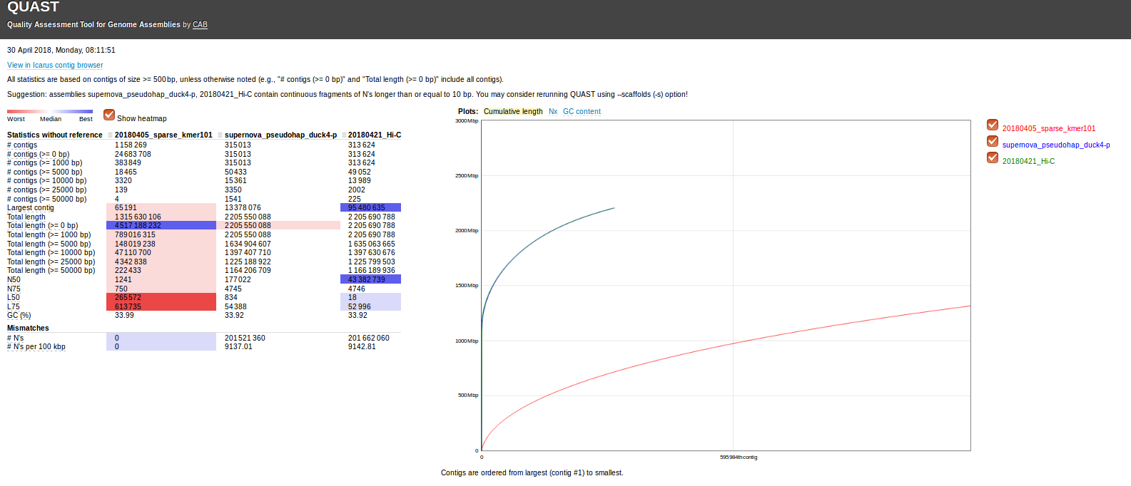
Assembly Stats – Geoduck Genome Assembly Comparisons w/Quast – SparseAssembler, SuperNova, Hi-C

Steven requested a comparison of geoduck genome assemblies.

Ran the following Quast command:

/home/sam/software/quast-4.5/quast.py \
-t 24 \
--labels 20180405_sparse_kmer101,supernova_pseudohap_duck4-p,20180421_Hi-C \
/mnt/owl/Athaliana/20180405_sparseassembler_kmer101_geoduck/Contigs.txt \
/mnt/owl//halfshell/bu-mox/analyses/0305b/duck4-p.fasta.gz \
/mnt/owl/Athaliana/20180419_geoduck_hi-c/Results/geoduck_roberts\ results\ 2018-04-21\ 18\:09\:04.514704/PGA_assembly.fasta
Results:

Quast output folder: results_2018_04_30_08_00_42/

Quast report (HTML): results_2018_04_30_08_00_42/report.html

The data’s pretty interesting and cool!

SparseAssembler has over 2x the amount of data (in bas pairs), yet produces the worst assembly.

SuperNova and Hi-C assemblies are very close in nearly all categories. This isn’t surprising, as the SuperNova assembly was used as a reference assembly for the Hi-C assembly.

However, the Hi-C assembly is insanely better than the SuperNova assembly! For example:

  • Largest contig is ~7x larger than the SuperNova assembly.
  • The N50 size is ~243x larger than the SuperNova assembly!!
  • L50 is only 18, 46x smaller than the SuperNova assembly!

This is pretty amazing, honestly. Even more amazing is that this data was sent over to us as some “preliminary” data for us to take a peak at!

Assembly Stats – Geoduck Hi-C Assembly Comparison

Ran the following Quast command to compare the two geoduck assemblies provided to us by Phase Genomics:

/home/sam/software/quast-4.5/quast.py \
-t 24 \
--labels 20180403_pga,20180421_pga \
/mnt/owl/Athaliana/20180421_geoduck_hi-c/Results/geoduck_roberts\ results\ 2018-04-03\ 11\:05\:41.596285/PGA_assembly.fasta \
/mnt/owl/Athaliana/20180421_geoduck_hi-c/Results/geoduck_roberts\ results\ 2018-04-21\ 18\:09\:04.514704/PGA_assembly.fasta
Results:

Quast Output folder: results_2018_04_30_11_16_04/

Quast report (HTML): results_2018_04_30_11_16_04/report.html

The two assemblies are nearly identical. Interesting…

DNA Isolation & Quantification – Metagenomics Water Filters

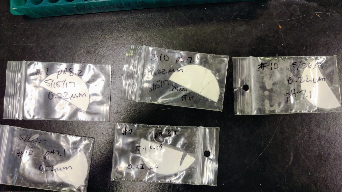
After discussing the preliminary DNA isolation attemp with Steven & Emma, we decided to proceed with DNA isolations on the remaining 0.22μm filters.

Isolated DNA from the following five filters:

DNA was isolated with the DNeasy Blood & Tissue Kit (Qiagen), following a modified version of the Gram-Positive Bacteria protocol:

  • filters were unfolded and unceremoniously stuffed into 1.7mL snap cap tubes
  • did not perform enzymatic lysis step
  • filters were incubated with 400μL of Buffer AL and 50μL of Proteinase K (both are double the volumes listed in the kit and are necessary to fully coat the filter in a 1.7mL snap cap tube)
  • 56oC incubations were performed overnight
  • 400μL of 100% ethanol was added to each after the 56oC incubation
  • samples were eluted in 50μL of Buffer AE
  • all spins were performed at 20,000g

Samples were quantified with the Roberts Lab Qubit 3.0 and the Qubit 1x dsDNA HS Assay Kit.

Used 5μL of each sample for measurement (see Results for update).

Results:

Raw data (Google Sheet): 20180426_qubit_metagenomics_filters

Sample Concentration(ng/μL) Initial_volume(μL) Yield(ng)
Filter #10 pH 7.1 5/15/17 0.296 50 14.65
Filter #7 pH 8.2 5/15/17 8.44 50 422
Filter #7 pH 8.2 5/1917 2.52 50 126
Filter #10 pH 7.1 5/22/17 2.0 50 100
Filter #10 pH 7.1 5/26/17 11.9 50 595

Samples were stored Sam gDNA Box #2, positions G8 – H3. (FTR 213, #27 (small -20oC frezer))

Total Alkalinity Calculations – Yaamini’s Ocean Chemistry Samples

I ran a subset of Yaamini’s ocean chemistry samples on our T5 Excellence titrator (Mettler Toledo) at the beginning of April. The subset were samples taken from the beginning, middle, and end of the experiment. The rationale for this was to assess whether or not total alkalinity (TA) varied across the experiment. If there was little variation, then there’d likely be no need to run all of the samples. However, should there be temporal differences, then all samples should be processed.

Data analysis was performed in the following R Project:

The R Project above was initially copied from the R Project for our titrator on GitHub:

Three separate, data-file-specific versions of the TA_calculations.R script were created and run:

Salinity values (PSU) were collected from the following spreadsheet (Google Sheet) and manually entered in each of the R scripts:

Specifically, the TA calculations were performed using the seacarb library, with the at() function.

Results:
sample_names TA_values (μmol/kg)
H1 A 2/20/17 2390.88423
H2 A 2/20/17 2393.39207
T1 A 2/20/17 2367.78791
T2 A 2/20/17 2319.39360
T3 A 2/20/17 2309.88602
T4 A 2/20/17 2287.72108
T5 A 2/20/17 2336.14773
T6 A 2/20/17 2298.36327
H1 A 3/20/17 2870.73309
H2 A 3/20/17 2760.49972
T1 A 3/20/17 2930.29308
T2 A 3/20/17 2925.95472
T3 A 3/20/17 2896.55123
T4 A 3/20/17 2769.72514
T5 A 3/20/17 2743.33934
T6 A 3/20/17 2727.94064
H1 A 4/4/17 2770.20971
H2 A 4/4/17 2656.27437
T1 A 4/4/17 2801.77913
T2 A 4/4/17 2822.51611
T3 A 4/4/17 2800.87387
T4 A 4/4/17 2584.60933
T5 A 4/4/17 2645.37017
T6 A 4/4/17 2604.22677

Well, it certainly looks like there’s some variation across the experiment. It’s likely that all remaining samples will need to be processed. Will pass along data to Yaamini for her to evaluate.

Assembly – SparseAssembler (k 111) on Geoduck Sequence Data

Continuing to try to find the best kmer setting to work with SparseAssemlber after the last attempt failed due to a kmer size that was too large (k 131; which happens to be outside the max kmer size [127] for SparseAssembler), I re-ran SparseAssembler with an arbitrarily selected kmer size < 131 (picked k 111).

The job was run on our Mox HPC node.

Results:

Output folder:

Slurm output file:

This failed with the following error message:

Error! K-mer size too large!

Well, this is disappointing. Not entirely sure why this is the case, as it’s below the max kmer setting for SparseAssembler. However, I’m not terribly surprised, as this happened previously (only using NovaSeq data) with a kmer setting of 117.

I’ve posted an issue on the kmergenie GitHub page; we’ll see what happens.